分成三個部分: Basic Plots, Vega, Gadfly,討論如何在 julia 進行 data visulization
Basic plots
使用 PyPlot,這是以 python matplotlib.pyplot module 提供的功能
使用前要先安裝 matplotlib
python -m pip install matplotlib在 julia 安裝 PyPlot
Pkg.add("PyPlot")用以下指令在 julia 測試 PyPlot
using PyPlot
x = 1:100
y = rand(100)
p = PyPlot.plot(x,y)
xlabel("x")
ylabel("y")
title("basic plot")
grid("true")
會得到這樣的圖形結果

另一個例子
using PyPlot

x = range(0, stop=4pi, length=1000)
y = cos.(pi .+ sin.(x))

xlabel("x-axis")
ylabel("y-axis")
title("using sin and cos functions")

plot(x, y, color="red")

XKCD 是一種 casual-style, handwritten graph mode
using PyPlot

x = [1:1:10;]
y = ones(10)

for i = 1:1:10
    y[i] = pi + i*i
end

xkcd()
xlabel("x-axis")
ylabel("y-axis")
title("XKCD")
plot(x,y)

bar chart
using PyPlot

x = [10,20,30,40,50]
y = [2,4,6,8,10]
xlabel("x-axis")
ylabel("y-axis")
title("Vertical bar graph")
bar(x, y, color="red")
horizontal bar chart
clf()
x = [10,20,30,40,50]
y = [2,4,6,8,10]
title("Horizontal bar graph")
xlabel("x-axis")
ylabel("y-axis")
barh(x,y,color="red")
2D histogram
clf()
x = rand(1000)
y = rand(1000)
xlabel("x-axis")
ylabel("y-axis")
title("2D Histograph")
hist2D(x, y, bins=50)
pie chart
clf()
labels = ["Fruits";"Vegetables";"Wheat"]
colors = ["Orange";"Blue";"Red"]
sizes = [25;40;35]
explode = zeros(length(sizes))
fig = figure("piechart", figsize=(10,10))
p = pie(sizes, labels=labels, shadow=true, startangle=90, colors = colors)
title("Pie charts")
Scatter chart
clf()
fig = figure("scatterplot", figsize = (10,10))
x = rand(50)
y = rand(50)
areas = 1000*rand(50);
scatter(x, y, s=areas, alpha=0.5)
xlabel("x-axis")
ylabel("y-axis")
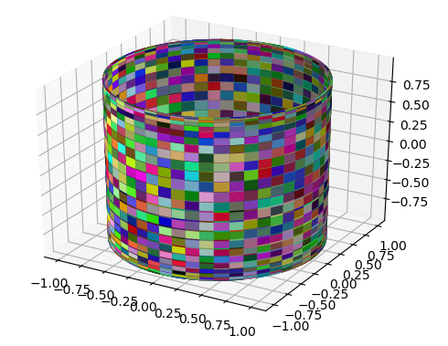
title("Scatter Plot")PyPlot 的 3D plot 是使用 surf(x, y, z, facecolors=colors)
| 參數 | 說明 |
|---|---|
| X,Y,Z | Data values as 2D arrays |
| rstride | Array row stride (step size) |
| cstride | Array column stride (step size) |
| rcount | Use at most this many rows, defaults to 50 |
| ccount | Use at most this many columns, defaults to 50 |
| color | Color of the surface patches |
| cmap | A colormap for the surface patches. |
| facecolors | Face colors for the individual patches |
| norm | An instance of Normalize to map values to colors |
| vmin | Minimum value to map |
| vmax | Maximum value to map |
| shade | Whether to shade the facecolors |
using PyPlot

clf()
a = range(0.0, stop=2pi, length=500)
b = range(0.0, stop=2pi, length=500)

len_a = length(a)
len_b = length(b)

x = ones(len_a, len_b)
y = ones(len_a, len_b)
z = ones(len_a, len_b)

for i=1:len_a
    for j=1:len_b
        x[i,j] = sin(a[i])
        y[i,j] = cos(a[i])
        z[i,j] = sin(b[j])
    end
end

colors = rand(len_a, len_b, 3)
fig = figure()
surf(x, y, z, facecolors=colors)
fig[:canvas][:draw]()
Gadfly
這是一個圖形的 library,可以輸出圖片為 SVG, PNG, PostScript, PDF,也可用 IJulia 運作,跟 DataFrames 緊密整合,提供 pan, zoom, toggle 的功能。執行 Gadfly.plot 後,browser 會打開一個 html 檔案,裡面是 svg 圖片。
Pkg.add("Gadfly")
using Gadfly
Gadfly.plot(x = rand(10), y=rand(10))
# 折線圖
Gadfly.plot(x = rand(10),y=rand(10), Geom.point, Geom.line)
Gadfly.plot(x=1:10, y=[10^n for n in rand(10)], Scale.y_sqrt, Geom.point, Geom.smooth, Guide.xlabel("x"), Guide.ylabel("y"), Guide.title("Graph with labels"))
Plotting DataFrames with Gadfly
使用 RDatasets (有一些範例資料) 產生 DataFrame for the plot function
折線圖
using RDatasets
Gadfly.plot(dataset("datasets", "iris"),
        x="SepalLength",
        y="SepalWidth",
        Geom.line)

Point Plot
Gadfly.plot(dataset("datasets", "iris"),
        x="SepalLength",
        y="SepalWidth",
        Geom.point)

plot a graph between SepalLength and SepalWidth

histogram
Gadfly.plot(x=randn(4000), Geom.histogram(bincount=100))

preceding showcased histogram
Gadfly.plot(dataset("mlmRev", "Gcsemv"),
        x = "Course", color="Gender", Geom.histogram)
沒有留言:
張貼留言