2021/3/15

濾波器設計

首先介紹濾波器的基本概念:窗函數。濾波器的設計分成 FIR, IIR 兩種,其中 FIR Filter 使用 Window Method,IIR Filter 則包含 Butterworth Filter, Chebyshev Type I Filter, Chebyshev Type II Filter, 及 Elliptic Filter

濾波器在 DSP 系統中,可用來選取或抑制某些頻率範圍的輸入訊號,藉以產生符合需求的輸出訊號。

由於有限長度的脈衝響應無法實現 ideal filter,在設計實際的濾波器時,通常是考慮濾波器的頻率響應是否符合事先定義的規格,同時容許頻率響應有些微誤差。

實際的 lowpass filter 其頻率響應應如下圖,通過頻帶 passband 的範圍介於 \(0 ~ ω_p\) 之間,理想的頻率響應為 1;抑制頻帶 stopband 的範圍介於 \(ω_s ~ \pi\) 之間,理想的頻率響應為 0。其中 \(ω_p\) 稱為通過頻帶邊緣頻率 Passband Edge Frequency,\(ω_s\) 稱為抑制頻帶邊緣頻率 Stopband Edge Frequency。

實際的 lowpass filter 的設計,通常在通過頻帶或抑制頻帶內,容許頻率響應有些許波動(誤差),其中\(δ_p\) 稱為通過頻帶波紋 (Passband Ripple),\(δ_s\) 稱為抑制頻帶波紋 (Stopband Ripple)。在 \(ω_p ~ ω_s\) 之間,則是容許頻率響應從 1 逐漸降為 0,稱為過渡頻帶 (Transition Band)

filter 的設計,主要包含以下步驟:

  1. 定義濾波器規格:根據 DSP 應用的需求,選取濾波器的種類,例如:lowpass, highpass, bandpass, bandstop 等等。然後定義濾波器的規格,包含:passbadn 與 stopband 的截止頻率、取樣頻率等等參數

  2. 選取濾波器的種類:選取 FIR 或 IIR 濾波器作為設計目標。通常 FIR Filter 為穩定系統,若選取 IIR Filter ,則需要進一步檢驗其穩定性。

  3. 求轉換函式:根據濾波器規格,求濾波器的轉換函式 H(z),例如 FIR Filter 的轉換函式為

    \(H(z) = b_0+b_1z^{-1}+...+b_Mz^{-M}\)

    IIR 濾波器的轉換函式為:

    \(H(z) = \frac{b_0+b_1z^{-1}+...+b_Mz^{-M}}{a_0+a_1z^{-1}+...+a_Nz^{-N}}\)

    這個步驟的目的是求濾波器的係數:\(\{a_k\} k=0,1,...,N\) 與 \(\{b_k\} k=0,1,...,M\)

  4. 實現濾波器:在完成設計後,可採用硬體或軟體方式實現。

Window Function

idea lowpass filter 在時間域的脈衝響應為無限序列,因此,為了實現有限的脈衝響應,同時近似理想的 lowpass filter,最直接的方法是 Window Method。也就是定義 Window Function,用來擷取有限的脈衝響應。

Window Function 定義為:介於某特定區間的數學函示,區間外的數值為 0

任意函數與 window function 相乘後,結果就像是透過窗戶觀察該函數一樣。在 DSP,window function 經常用來進行頻譜分析、濾波器設計、音頻壓縮等等。

以下是幾個典型的 window function,這幾種 window function 都具有對稱性,SciPy 的Signal 有支援這些 functions。在濾波器設計過程中,窗函數通常是先經過平移,平移後以原點為中心,且對原點對稱,再與無限脈衝響應進行運算,藉以擷取有限的離散序列。

  • 矩形窗 Rectangular Window

    \( W(n) = \left\{ \begin{array}{ll} 1 & \mbox{if 0 ≤ n ≤ M-1} \\ 0 & \mbox{otherwise} \end{array} \right.\)

    其中 window 的大小為 M。由於矩形窗的形狀如同箱型車 boxcar,因此也被稱為 boxcar function

  • Hamming 窗

    \( W(n) = \left\{ \begin{array}{ll} 0.54-0.46cos(\frac{2 \pi n}{M-1}) & \mbox{if 0 ≤ n ≤ M-1} \\ 0 & \mbox{otherwise} \end{array} \right.\)

    這是根據 Richard W. Hamming 而命名的

  • Hanning 窗

    \( W(n) = \left\{ \begin{array}{ll} 0.5-0.5cos(\frac{2 \pi n}{M-1}) & \mbox{if 0 ≤ n ≤ M-1} \\ 0 & \mbox{otherwise} \end{array} \right.\)

    這是根據 Julus von Hann 而命名的,形狀跟 Hamming 窗相似

  • Bartlet 窗

    \( W(n) = \left\{ \begin{array}{ll} \frac{2}{M-1}(\frac{M-1}{2} - |n-\frac{M-1}{2}|) & \mbox{if 0 ≤ n ≤ M-1} \\ 0 & \mbox{otherwise} \end{array} \right.\)

    Bartlet window 的形狀是三角形

  • Blackman 窗

    \( W(n) = \left\{ \begin{array}{ll} 0.42-0.5cos(\frac{2 \pi n}{M-1})+0.08cos(\frac{4 \pi n}{M-1}) & \mbox{if 0 ≤ n ≤ M-1} \\ 0 & \mbox{otherwise} \end{array} \right.\)

    這是根據 Ralph B. Blackmand 而命名的

  • Kaiser 窗

    \(W(n) = I_0(β\sqrt{1-\frac{4n^2}{(M-1)^2}})/I_0(β), -\frac{M-1}{2} ≤ n ≤ \frac{M-1}{2}\)

    這是根據 Jim Kaiser 命名的。

    \(I_0\) 是修正的零階 Bessel 函式,參數 β 可用來近似其他窗函式。例如:β=0 為矩形窗、β=5 近似 Hamming 窗、β=6 近似 Hanning 窗、β=8.6 近似 Blackman 窗、β=14 則是 Kaiser 窗的建議初始值

統一選取 M=2*32+1 = 65,為有限脈衝響應的長度。window function 為對稱圖形,可平移到以原點為中心。

import numpy as np
import scipy.signal as signal
import matplotlib.pyplot as plt

M = 65
w1 = signal.boxcar( M )
w2 = signal.hamming( M )
w3 = signal.hann( M )
w4 = signal.bartlett( M )
w5 = signal.barthann( M )
w6 = signal.kaiser( M, 14 )

plt.subplot(231)
plt.plot( w1 )
plt.xlabel( 'n (rectangular, boxcar)' )
plt.ylabel( 'Amplitude' )

plt.subplot(232)
plt.plot( w2 )
plt.xlabel( 'n (hamming)' )
plt.ylabel( 'Amplitude' )

plt.subplot(233)
plt.plot( w3 )
plt.xlabel( 'n (hanning)' )
plt.ylabel( 'Amplitude' )

plt.subplot(234)
plt.plot( w4 )
plt.xlabel( 'n (bartlett)' )
plt.ylabel( 'Amplitude' )

plt.subplot(235)
plt.plot( w5 )
plt.xlabel( 'n (blackman)' )
plt.ylabel( 'Amplitude' )

plt.subplot(236)
plt.plot( w6 )
plt.xlabel( 'n (kaiser)' )
plt.ylabel( 'Amplitude' )

plt.show( )

FIR 濾波器設計

最簡單的方法是 window method,步驟如下

  1. 選取濾波器的種類:包含 lowpass, highpass, bandpass, bandstop 濾波器
  2. 定義濾波器的規格:如果是 lowpass, highpass,需定義截止頻率 (cutoff frequency),以 Hz 為單位,如果是 bandpass, bandstop,需定義兩個截止頻率
  3. 選取取樣頻率:sampling frequency,以 Hz 為單位。選取原則以輸入數位訊號為主,且對應的 Nyquist 頻率需大於上述的截止頻率
  4. 套用窗法:選取 window function。在此需選取濾波器的長度,也就是離散時間域的脈衝響應樣本數 (number of taps)
  5. FIR 濾波器係數:根據濾波器的種類,計算 FIR filter 的係數,並套用 window function,藉以擷取有限長度的脈衝響應。理論上,樣本數越多,越接近 ideal filter
  6. 頻率響應:根據脈衝響應,求其在頻率域的頻率響應,包含強度頻譜與相位頻譜,用來觀察濾波器的設計,是否符合原先地定義的規格需求

ex: 試用 window method 設計濾波器規格為

(1) lowpass filter:截止頻率 \(f_c=250Hz\)

(2) highpass filter:截止頻率 \(f_c=250Hz\)

(3) bandpass filter:截止頻率 \(f_1=200Hz, f_2=300Hz\)

(4) bandstop filter:截止頻率 \(f_1=200Hz, f_2=300Hz\)

並顯示強度頻率與相位頻譜


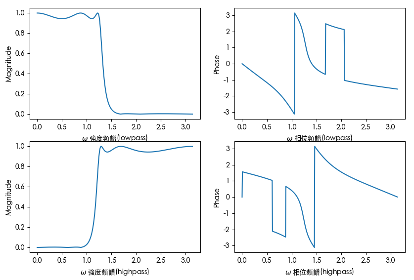
以下是用不同 window method 實作 lowpass filter 的結果

import numpy as np
import scipy.signal as signal
import matplotlib.pyplot as plt

def fir_filter(n, cutoff, win, pass_zero, freq, plotpos1, plotpos2):
    h = signal.firwin( n, cutoff, window = win, pass_zero = pass_zero, fs = freq )

    w, H = signal.freqz( h )
    magnitude = abs( H )
    phase = np.angle( H )

    plt.subplot(plotpos1)
    plt.plot( w, magnitude )
    plt.xlabel( r'$\omega$ '+'強度頻譜 ('+str(win)+')' )
    plt.ylabel( 'Magnitude' )

    plt.subplot(plotpos2)
    plt.plot( w, phase )
    plt.xlabel( r'$\omega$ '+'相位頻譜 ('+str(win)+')' )
    plt.ylabel( 'Phase' )

# cutoff frequency(Hz)
cutoff = 250
# numeber of taps
n = 31
# pass_zero = {True, False, 'bandpass', 'lowpass', 'highpass', 'bandstop'}
pass_zero = 'lowpass'
# sampling frequency (Hz)
freq = 1000


# 替換中文字型,處理 matplotlib 中文 label 問題
# https://blog.csdn.net/gmr2453929471/article/details/78655834
plt.rcParams['font.sans-serif'] = ['Heiti TC'] # 步驟一(替換sans-serif字型)
plt.rcParams['axes.unicode_minus'] = False  # 步驟二(解決座標軸負數的負號顯示問題)

plt.figure( 1 )

# rectangular (boxcar) window method
win='boxcar'
fir_filter(n, cutoff, win, pass_zero, freq, 231, 234)

# hamming window method
win='hamming'
fir_filter(n, cutoff, win, pass_zero, freq, 232, 235)

# hanning window method
win='hanning'
fir_filter(n, cutoff, win, pass_zero, freq, 233, 236)

plt.figure( 2 )

# bartlett window method
win='bartlett'
fir_filter(n, cutoff, win, pass_zero, freq, 231, 234)

# blackman window method
win='blackman'
fir_filter(n, cutoff, win, pass_zero, freq, 232, 235)

# kaiser window method
win=('kaiser',14)
fir_filter(n, cutoff, win, pass_zero, freq, 233, 236)

plt.show( )

使用 rectangular window method 設計的 lowpass filter,其頻率響應有 Gibbs 現象,結果較不理想。使用 blackman 或kaiser 設計的 lowpass filter,結果較理想。

截止角頻率經過正規化為 \(2 \pi f_c/f_s = 2 \pi (250) / 1000 = \pi/2\),角頻率介於 \(0~\pi\) 之間


以下是用 hamming window method 實作四種 filter 的結果

import numpy as np
import scipy.signal as signal
import matplotlib.pyplot as plt

def fir_filter(n, cutoff, win, pass_zero, freq, plotpos1):
    h = signal.firwin( n, cutoff, window = win, pass_zero = pass_zero, fs = freq )

    w, H = signal.freqz( h )
    magnitude = abs( H )
    phase = np.angle( H )

    plt.subplot(plotpos1)
    plt.plot( w, magnitude )
    plt.xlabel( r'$\omega$ '+'('+str(pass_zero)+')' )
    plt.ylabel( 'Magnitude' )

    # plt.subplot(plotpos2)
    # plt.plot( w, phase )
    # plt.xlabel( r'$\omega$ '+'相位頻譜 ('+str(win)+')' )
    # plt.ylabel( 'Phase' )

# cutoff frequency(Hz)
cutoff = 250
f1 = 200
f2 = 300

# numeber of taps
n = 31
# sampling frequency (Hz)
freq = 1000

# hamming window method
win='hamming'

plt.figure( 1 )

# lowpass
# pass_zero = {True, False, 'bandpass', 'lowpass', 'highpass', 'bandstop'}
pass_zero='lowpass'
fir_filter(n, cutoff, win, pass_zero, freq, 221)

pass_zero='highpass'
fir_filter(n, cutoff, win, pass_zero, freq, 222)

pass_zero='bandpass'
fir_filter(n, [f1, f2], win, pass_zero, freq, 223)

pass_zero='bandstop'
fir_filter(n, [f1, f2], win, pass_zero, freq, 224)

plt.show( )

IIR 濾波器設計

IIR filters 分為以下幾種

  1. Butterworth Filter
  2. Chebyshev Type I Filter
  3. Chebyshev Type II Filter
  4. Elliptic Filter 橢圓濾波器

IIR filter 的設計步驟,跟 FIR filter 的步驟類似

  1. 選取濾波器的種類:包含 lowpass, highpass, bandpass, bandstop 濾波器

  2. 定義濾波器的規格:如果是 lowpass, highpass,需定義截止頻率 (cutoff frequency),以 Hz 為單位,如果是 bandpass, bandstop,需定義兩個截止頻率。另外需要定義通過頻帶波紋與抑制頻帶波紋,單位為 dB

  3. 選取取樣頻率:sampling frequency,以 Hz 為單位。選取原則以輸入數位訊號為主,且對應的 Nyquist 頻率需大於上述的截止頻率

  4. 濾波器參數:根據濾波器的規格,計算濾波器的階數 (Order) 與 -3dB 截止頻率

  5. IIR 濾波器係數:根據濾波器的種類及相關參數,計算轉換函式

    \(H(z)=\frac{Y(z)}{X(z)} = \frac{b_0+b_1z^{-1}+...+b_Mz^{-M}}{a_0+z_1z^{-1}+...+a_Nz^{-N}}\)

    也就是計算濾波器的係數 \(\{a_k\}, k=1,2,...,N\) \(\{b_k\}, k=0,1,...M\)

  6. 頻率響應:根據脈衝響應,求其在頻率域的頻率響應,包含強度頻譜與相位頻譜,用來觀察濾波器的設計,是否符合原先地定義的規格需求

Butterworth 濾波器

是一種通過頻帶的頻率響應非常平坦的 DSP,由英國工程師 Stephen Butterworth 提出

根據下列規格,設計 Butterworth filters

(1) lowpass filter & highpass filter

通過頻帶邊緣頻率 200 Hz

抑制頻帶邊緣頻率 300 Hz

通過頻帶波紋 0.5 dB

抑制頻帶波紋 50 dB

取樣頻率 1000Hz

(2) bandpass & bandstop filter

通過頻帶邊緣頻率 200, 300 Hz

抑制頻帶邊緣頻率 100, 400 Hz

通過頻帶波紋 0.5 dB

抑制頻帶波紋 50 dB

取樣頻率 1000Hz

import numpy as np
import scipy.signal as signal
import matplotlib.pyplot as plt

def plot(a, b, plotname, plotpos1, plotpos2):
    w, H = signal.freqz( b, a )
    magnitude = abs( H )
    phase = np.angle( H )

    plt.subplot(plotpos1)
    plt.plot( w, magnitude )
    plt.xlabel( r'$\omega$ 強度頻譜('+plotname+')' )
    plt.ylabel( 'Magnitude' )

    plt.subplot(plotpos2)
    plt.plot( w, phase )
    plt.xlabel( r'$\omega$ 相位頻譜('+plotname+')' )
    plt.ylabel( 'Phase' )

# 替換中文字型,處理 matplotlib 中文 label 問題
# https://blog.csdn.net/gmr2453929471/article/details/78655834
plt.rcParams['font.sans-serif'] = ['Heiti TC'] # 步驟一(替換sans-serif字型)
plt.rcParams['axes.unicode_minus'] = False  # 步驟二(解決座標軸負數的負號顯示問題)


# lowpass filter
# passband edge frequency(Hz)
fp = 200
# stopband edge frequency(Hz)
fs = 300
# passband ripple(dB)
rp = 0.5
# stopband ripple(dB)
rs = 50
# sampling frequency
Fs = 1000

wp = 2 * fp / Fs
ws = 2 * fs / Fs

n, wn = signal.buttord( wp, ws, rp, rs )
b, a = signal.butter( n, wn, 'lowpass' )

plt.figure( 1 )
plot(a, b, 'lowpass', '121', '122')


# highpass filter
# passband edge frequency(Hz)
fp = 200
# stopband edge frequency(Hz)
fs = 300
# passband ripple(dB)
rp = 0.5
# stopband ripple(dB)
rs = 50
# sampling frequency
Fs = 1000

wp = 2 * fp / Fs
ws = 2 * fs / Fs

n, wn = signal.buttord( wp, ws, rp, rs )
b, a = signal.butter( n, wn, 'highpass' )

plt.figure( 2 )
plot(a, b, 'highpass', '121', '122')


# bandpass filter
# 1st passband edge frequency(Hz)
fp1 = 200
# 2nd passband edge frequency(Hz)
fp2 = 300
# 1st stopband edge frequency(Hz)
fs1 = 100
# 2nd stopband edge frequency(Hz)
fs2 = 400
# passband ripple(dB)
rp = 0.5
# stopband ripple(dB)
rs = 50
# sampling frequency
Fs = 1000

wp1 = 2 * fp1 / Fs
wp2 = 2 * fp2 / Fs
ws1 = 2 * fs1 / Fs
ws2 = 2 * fs2 / Fs

n, wn = signal.buttord( [wp1, wp2], [ws1, ws2], rp, rs )
b, a = signal.butter( n, wn, 'bandpass' )

plt.figure( 3 )
plot(a, b, 'bandpass', '121', '122')


# bandstop filter
# 1st passband edge frequency(Hz)
fp1 = 200
# 2nd passband edge frequency(Hz)
fp2 = 300
# 1st stopband edge frequency(Hz)
fs1 = 100
# 2nd stopband edge frequency(Hz)
fs2 = 400
# passband ripple(dB)
rp = 0.5
# stopband ripple(dB)
rs = 50
# sampling frequency
Fs = 1000

wp1 = 2 * fp1 / Fs
wp2 = 2 * fp2 / Fs
ws1 = 2 * fs1 / Fs
ws2 = 2 * fs2 / Fs

n, wn = signal.buttord( [wp1, wp2], [ws1, ws2], rp, rs )
b, a = signal.butter( n, wn, 'bandstop' )

plt.figure( 4 )
plot(a, b, 'bandstop', '121', '122')

plt.show( )

Chebyshev Type I Filter

Chebyshev Filter 是一種在通過頻帶或抑制頻帶上頻率響應等波動的濾波器。在通過頻帶波動的濾波器為 Chebyshev Type I Filter,在抑制頻帶上波動的濾波器為 Chebyshev Type II Filter

根據下列規格,設計 Chebyshev Type I Filters

(1) lowpass filter & highpass filter

通過頻帶邊緣頻率 200 Hz

抑制頻帶邊緣頻率 300 Hz

通過頻帶波紋 0.5 dB

抑制頻帶波紋 50 dB

取樣頻率 1000Hz

(2) bandpass & bandstop filter

通過頻帶邊緣頻率 200, 300 Hz

抑制頻帶邊緣頻率 100, 400 Hz

通過頻帶波紋 0.5 dB

抑制頻帶波紋 50 dB

取樣頻率 1000Hz

import numpy as np
import scipy.signal as signal
import matplotlib.pyplot as plt

def plot(a, b, plotname, plotpos1, plotpos2):
    w, H = signal.freqz( b, a )
    magnitude = abs( H )
    phase = np.angle( H )

    plt.subplot(plotpos1)
    plt.plot( w, magnitude )
    plt.xlabel( r'$\omega$ 強度頻譜('+plotname+')' )
    plt.ylabel( 'Magnitude' )

    plt.subplot(plotpos2)
    plt.plot( w, phase )
    plt.xlabel( r'$\omega$ 相位頻譜('+plotname+')' )
    plt.ylabel( 'Phase' )

# 替換中文字型,處理 matplotlib 中文 label 問題
# https://blog.csdn.net/gmr2453929471/article/details/78655834
plt.rcParams['font.sans-serif'] = ['Heiti TC'] # 步驟一(替換sans-serif字型)
plt.rcParams['axes.unicode_minus'] = False  # 步驟二(解決座標軸負數的負號顯示問題)

# lowpass filter
# passband edge frequency(Hz)
fp = 200
# stopband edge frequency(Hz)
fs = 300
# passband ripple(dB)
rp = 0.5
# stopband ripple(dB)
rs = 50
# sampling frequency
Fs = 1000

wp = 2 * fp / Fs
ws = 2 * fs / Fs

n, wn = signal.cheb1ord( wp, ws, rp, rs )
b, a = signal.cheby1( n, rp, wn, 'lowpass' )

plt.figure( 1 )
plot(a, b, 'lowpass', '221', '222')


# highpass filter
# passband edge frequency(Hz)
fp = 200
# stopband edge frequency(Hz)
fs = 300
# passband ripple(dB)
rp = 0.5
# stopband ripple(dB)
rs = 50
# sampling frequency
Fs = 1000

wp = 2 * fp / Fs
ws = 2 * fs / Fs

n, wn = signal.cheb1ord( wp, ws, rp, rs )
b, a = signal.cheby1( n, rp, wn, 'highpass' )

plot(a, b, 'highpass', '223', '224')


# bandpass filter
# 1st passband edge frequency(Hz)
fp1 = 200
# 2nd passband edge frequency(Hz)
fp2 = 300
# 1st stopband edge frequency(Hz)
fs1 = 100
# 2nd stopband edge frequency(Hz)
fs2 = 400
# passband ripple(dB)
rp = 0.5
# stopband ripple(dB)
rs = 50
# sampling frequency
Fs = 1000

wp1 = 2 * fp1 / Fs
wp2 = 2 * fp2 / Fs
ws1 = 2 * fs1 / Fs
ws2 = 2 * fs2 / Fs

n, wn = signal.cheb1ord( [ wp1, wp2 ], [ ws1, ws2 ], rp, rs )
b, a = signal.cheby1( n, rp, wn, 'bandpass' )

plt.figure( 2 )
plot(a, b, 'bandpass', '221', '222')


# bandstop filter
# 1st passband edge frequency(Hz)
fp1 = 200
# 2nd passband edge frequency(Hz)
fp2 = 300
# 1st stopband edge frequency(Hz)
fs1 = 100
# 2nd stopband edge frequency(Hz)
fs2 = 400
# passband ripple(dB)
rp = 0.5
# stopband ripple(dB)
rs = 50
# sampling frequency
Fs = 1000

wp1 = 2 * fp1 / Fs
wp2 = 2 * fp2 / Fs
ws1 = 2 * fs1 / Fs
ws2 = 2 * fs2 / Fs

n, wn = signal.cheb1ord( [ wp1, wp2 ], [ ws1, ws2 ], rp, rs )
b, a = signal.cheby1( n, rp, wn, 'bandstop' )

plot(a, b, 'bandstop', '223', '224')

plt.show( )

Chebyshev Type II Filter

在抑制頻帶上波動的濾波器為 Chebyshev Type II Filter

根據下列規格,設計 Chebyshev Type II Filters

(1) lowpass filter & highpass filter

通過頻帶邊緣頻率 200 Hz

抑制頻帶邊緣頻率 300 Hz

通過頻帶波紋 0.5 dB

抑制頻帶波紋 50 dB

取樣頻率 1000Hz

(2) bandpass & bandstop filter

通過頻帶邊緣頻率 200, 300 Hz

抑制頻帶邊緣頻率 100, 400 Hz

通過頻帶波紋 0.5 dB

抑制頻帶波紋 50 dB

取樣頻率 1000Hz

import numpy as np
import scipy.signal as signal
import matplotlib.pyplot as plt

def plot(a, b, plotname, plotpos1, plotpos2):
    w, H = signal.freqz( b, a )
    magnitude = abs( H )
    phase = np.angle( H )

    plt.subplot(plotpos1)
    plt.plot( w, magnitude )
    plt.xlabel( r'$\omega$ 強度頻譜('+plotname+')' )
    plt.ylabel( 'Magnitude' )

    plt.subplot(plotpos2)
    plt.plot( w, phase )
    plt.xlabel( r'$\omega$ 相位頻譜('+plotname+')' )
    plt.ylabel( 'Phase' )

# 替換中文字型,處理 matplotlib 中文 label 問題
# https://blog.csdn.net/gmr2453929471/article/details/78655834
plt.rcParams['font.sans-serif'] = ['Heiti TC'] # 步驟一(替換sans-serif字型)
plt.rcParams['axes.unicode_minus'] = False  # 步驟二(解決座標軸負數的負號顯示問題)

# lowpass filter
# passband edge frequency(Hz)
fp = 200
# stopband edge frequency(Hz)
fs = 300
# passband ripple(dB)
rp = 0.5
# stopband ripple(dB)
rs = 50
# sampling frequency
Fs = 1000

wp = 2 * fp / Fs
ws = 2 * fs / Fs

n, wn = signal.cheb2ord( wp, ws, rp, rs )
b, a = signal.cheby2( n, rp, wn, 'lowpass' )

plt.figure( 1 )
plot(a, b, 'lowpass', '221', '222')


# highpass filter
# passband edge frequency(Hz)
fp = 200
# stopband edge frequency(Hz)
fs = 300
# passband ripple(dB)
rp = 0.5
# stopband ripple(dB)
rs = 50
# sampling frequency
Fs = 1000

wp = 2 * fp / Fs
ws = 2 * fs / Fs

n, wn = signal.cheb2ord( wp, ws, rp, rs )
b, a = signal.cheby2( n, rp, wn, 'highpass' )

plot(a, b, 'highpass', '223', '224')


# bandpass filter
# 1st passband edge frequency(Hz)
fp1 = 200
# 2nd passband edge frequency(Hz)
fp2 = 300
# 1st stopband edge frequency(Hz)
fs1 = 100
# 2nd stopband edge frequency(Hz)
fs2 = 400
# passband ripple(dB)
rp = 0.5
# stopband ripple(dB)
rs = 50
# sampling frequency
Fs = 1000

wp1 = 2 * fp1 / Fs
wp2 = 2 * fp2 / Fs
ws1 = 2 * fs1 / Fs
ws2 = 2 * fs2 / Fs

n, wn = signal.cheb2ord( [ wp1, wp2 ], [ ws1, ws2 ], rp, rs )
b, a = signal.cheby2( n, rp, wn, 'bandpass' )

plt.figure( 2 )
plot(a, b, 'bandpass', '221', '222')


# bandstop filter
# 1st passband edge frequency(Hz)
fp1 = 200
# 2nd passband edge frequency(Hz)
fp2 = 300
# 1st stopband edge frequency(Hz)
fs1 = 100
# 2nd stopband edge frequency(Hz)
fs2 = 400
# passband ripple(dB)
rp = 0.5
# stopband ripple(dB)
rs = 50
# sampling frequency
Fs = 1000

wp1 = 2 * fp1 / Fs
wp2 = 2 * fp2 / Fs
ws1 = 2 * fs1 / Fs
ws2 = 2 * fs2 / Fs

n, wn = signal.cheb2ord( [ wp1, wp2 ], [ ws1, ws2 ], rp, rs )
b, a = signal.cheby2( n, rp, wn, 'bandstop' )

plot(a, b, 'bandstop', '223', '224')

plt.show( )

Elliptic Filter

是一種在通過頻帶與抑制頻帶波紋的濾波器。橢圓濾波器比其他類型的濾波器,在階數相同的條件下,有比較小的通過頻帶與抑制頻帶波動。

根據下列規格,設計 Elliptic Filters

(1) lowpass filter & highpass filter

通過頻帶邊緣頻率 200 Hz

抑制頻帶邊緣頻率 300 Hz

通過頻帶波紋 0.5 dB

抑制頻帶波紋 50 dB

取樣頻率 1000Hz

(2) bandpass & bandstop filter

通過頻帶邊緣頻率 200, 300 Hz

抑制頻帶邊緣頻率 100, 400 Hz

通過頻帶波紋 0.5 dB

抑制頻帶波紋 50 dB

取樣頻率 1000Hz

import numpy as np
import scipy.signal as signal
import matplotlib.pyplot as plt

def plot(a, b, plotname, plotpos1, plotpos2):
    w, H = signal.freqz( b, a )
    magnitude = abs( H )
    phase = np.angle( H )

    plt.subplot(plotpos1)
    plt.plot( w, magnitude )
    plt.xlabel( r'$\omega$ 強度頻譜('+plotname+')' )
    plt.ylabel( 'Magnitude' )

    plt.subplot(plotpos2)
    plt.plot( w, phase )
    plt.xlabel( r'$\omega$ 相位頻譜('+plotname+')' )
    plt.ylabel( 'Phase' )

# 替換中文字型,處理 matplotlib 中文 label 問題
# https://blog.csdn.net/gmr2453929471/article/details/78655834
plt.rcParams['font.sans-serif'] = ['Heiti TC'] # 步驟一(替換sans-serif字型)
plt.rcParams['axes.unicode_minus'] = False  # 步驟二(解決座標軸負數的負號顯示問題)

# lowpass filter
# passband edge frequency(Hz)
fp = 200
# stopband edge frequency(Hz)
fs = 300
# passband ripple(dB)
rp = 0.5
# stopband ripple(dB)
rs = 50
# sampling frequency
Fs = 1000

wp = 2 * fp / Fs
ws = 2 * fs / Fs

n, wn = signal.ellipord( wp, ws, rp, rs )
b, a = signal.ellip( n, rp, rs, wn, 'lowpass' )

plt.figure( 1 )
plot(a, b, 'lowpass', '221', '222')


# highpass filter
# passband edge frequency(Hz)
fp = 200
# stopband edge frequency(Hz)
fs = 300
# passband ripple(dB)
rp = 0.5
# stopband ripple(dB)
rs = 50
# sampling frequency
Fs = 1000

wp = 2 * fp / Fs
ws = 2 * fs / Fs

n, wn = signal.ellipord( wp, ws, rp, rs )
b, a = signal.ellip( n, rp, rs, wn, 'highpass' )

plot(a, b, 'highpass', '223', '224')


# bandpass filter
# 1st passband edge frequency(Hz)
fp1 = 200
# 2nd passband edge frequency(Hz)
fp2 = 300
# 1st stopband edge frequency(Hz)
fs1 = 100
# 2nd stopband edge frequency(Hz)
fs2 = 400
# passband ripple(dB)
rp = 0.5
# stopband ripple(dB)
rs = 50
# sampling frequency
Fs = 1000

wp1 = 2 * fp1 / Fs
wp2 = 2 * fp2 / Fs
ws1 = 2 * fs1 / Fs
ws2 = 2 * fs2 / Fs

n, wn = signal.ellipord( [ wp1, wp2 ], [ ws1, ws2 ], rp, rs )
b, a = signal.ellip( n, rp, rs, wn, 'bandpass' )

plt.figure( 2 )
plot(a, b, 'bandpass', '221', '222')


# bandstop filter
# 1st passband edge frequency(Hz)
fp1 = 200
# 2nd passband edge frequency(Hz)
fp2 = 300
# 1st stopband edge frequency(Hz)
fs1 = 100
# 2nd stopband edge frequency(Hz)
fs2 = 400
# passband ripple(dB)
rp = 0.5
# stopband ripple(dB)
rs = 50
# sampling frequency
Fs = 1000

wp1 = 2 * fp1 / Fs
wp2 = 2 * fp2 / Fs
ws1 = 2 * fs1 / Fs
ws2 = 2 * fs2 / Fs

n, wn = signal.ellipord( [ wp1, wp2 ], [ ws1, ws2 ], rp, rs )
b, a = signal.ellip( n, rp, rs, wn, 'bandstop' )

plot(a, b, 'bandstop', '223', '224')

plt.show( )
References

數位訊號處理:Python程式實作(附範例光碟)(第二版)

2021/3/8

頻率域 DSP

頻率域的數位訊號處理 Digital Signal Processing in Frequency Domain

到目前為止,DSP 是以離散時間域的數學運算為主軸,例如:卷積運算、移動平均濾波器、FIR 濾波器、IIR 濾波器。本章是以頻率域的數位訊號處理為主軸

頻率域 DSP 的系統方塊圖

處理步驟如下:

  1. 輸入的數位訊號 x[n],取離散時間傅立葉轉換 DTFT,結果為

    \(X(e^{jω}) = F\{x[n]\}\)

    在DSP 實務中,則是採用離散傅立葉轉換 (Discrete Fourier Transform, DFT),即

    \(X[k] = \sum_{n=0}^{N-1}x[n]e^{-j2 \pi kn/N}, k=0,1,...,N-1\)

    為了縮短處理時間,通常採用快速傅立葉轉換 Fast Fourier Transform, FFT 的演算法進行運算。注意運算結果為複數陣列

  2. 根據系統輸入/輸出的目的或規格,進行濾波器的設計,藉以產生頻率響應,即

    \(H(e^{jω}) = F\{h[n]\}\)

    在 DSP 實務中,根據濾波器的種類,設計濾波器的頻率響應 Frequency Response,通常頻率響應在特定頻率範圍的響應值(或強度值),介於 0~1 之間

  3. 套用濾波器,通常使用卷積定理,藉以產生輸出訊號的頻率域表示法

    \(Y(e^{jω}) = H(e^{jω})X(e^{jω})\)

    在 DSP 實務中,運用陣列的點對點乘法 (Pointwise Multiplication) 運算,達到濾波的效果,即

    \(Y[k] = H[k] \cdot X[k]\)

    結果通常是複數陣列

  4. 最後,取反離散時間傅立葉轉換(Inverse DTFT),即可得到輸出訊號

    \(y[n] = F^{-1}\{Y(e^{jω})\}\)

    在 DSP 實務中,採用反離散傅立葉轉換 Inverse DFT,即

    \(y[n] = \frac{1}{N} \sum_{k=0}^{N-1} Y[k]e^{j2 \pi kn/N}, n=0,1,2,...,N-1\)

    在此,也是使用反快速傅立葉轉換 Inverse FFT,縮短處理時間。由於處理後的結果為複數,通常是取實數部分(忽略虛數),作為輸出訊號,必要時,進一步將數值作正規化處理,藉以控制輸出訊號的數值範圍

理想濾波器

理想濾波器在離散時間域的脈衝響應是有限數列,因此無法在離散時間域實現理想濾波器,然而透過頻率域 DSP,可實現理想濾波器。

ex: 輸入訊號諧波定義如下

\(x(t) = cos(2 \pi \cdot 10 \cdot t)+ cos(2 \pi \cdot 20 \cdot t) + cos(2 \pi \cdot 30 \cdot t)\)

取樣頻率 \(f_s=500Hz\),試套用以下理想濾波器

(1) 理想低通濾波器,截止頻率 \(f_c=15Hz\)

(2) 理想高通濾波器,截止頻率 \(f_c=15Hz\)

(3) 理想帶通濾波器,截止頻率 \(f_1=15Hz, f_2=25Hz\)

(4) 理想帶阻濾波器,截止頻率 \(f_1=15Hz, f_2=25Hz\)

import numpy as np
from numpy.fft import fft, fftshift, ifft, fftfreq
import matplotlib.pyplot as plt

def ideal_lowpass_filtering( x, cutoff, fs ):
    X = fft( x )
    H = np.zeros( fs )
    for i in range( -cutoff, cutoff + 1 ):
        H[i] = 1
    Y = H * X
    y = ifft( Y )
    y = y.real
    return y

def ideal_highpass_filtering( x, cutoff, fs ):
    X = fft( x )
    H = np.zeros( fs )
    for i in range( -cutoff, cutoff + 1 ):
        H[i] = 1
    H = 1 - H
    Y = H * X
    y = ifft( Y )
    y = y.real
    return y

def ideal_bandpass_filtering( x, f1, f2, fs ):
    X = fft( x )
    H = np.zeros( fs )
    for i in range( f1, f2 + 1 ):
        H[i] = 1
    for i in range( -f1, -f2 - 1, -1 ):
        H[i] = 1
    Y = H * X
    y = ifft( Y )
    y = y.real
    return y

def ideal_bandstop_filtering( x, f1, f2, fs ):
    X = fft( x )
    H = np.zeros( fs )
    for i in range( f1, f2 + 1 ):
        H[i] = 1
    for i in range( -f1, -f2 - 1, -1 ):
        H[i] = 1
    H = 1 - H
    Y = H * X
    y = ifft( Y )
    y = y.real
    return y

def ideal_allpass_filtering( x ):
    X = fft( x )
    Y = X
    y = ifft( Y )
    y = y.real
    return y

def main( ):
    # print( "DSP in Frequency Domain" )
    # print( "(1) Ideal Lowpass Filtering" )
    # print( "(2) Ideal Highpass Filtering" )
    # print( "(3) Ideal Bandpass Filtering" )
    # print( "(4) Ideal Bandstop Filtering" )
    # print( "(5) Ideal Allpass Filtering" )

    # choice = eval( input( "Please enter your choice: " ) )

    # if choice == 1 or choice == 2:
    #   fc = eval( input( "Please enter cutoff frequency(Hz): " ) )

    # if choice == 3 or choice == 4:
    #   f1 = eval( input( "Please enter frequency f1(Hz): " ) )
    #   f2 = eval( input( "Please enter frequency f2(Hz): " ) )

    fc = 15

    f1 = 15
    f2 = 25

    # 取樣頻率
    fs = 500
    t = np.linspace( 0, 1, fs, endpoint = False )
    # 原始訊號 (諧波)
    x = np.cos( 2 * np.pi * 10 * t ) + np.cos( 2 * np.pi * 20 * t ) + np.cos( 2 * np.pi * 30 * t )

    # fftfreq: 離散傅立葉轉換的採樣頻率
    # fftshift: 將 0 移到正中心
    f = fftshift( fftfreq( fs, 1 / fs ) )
    Xm = abs( fftshift( fft( x ) ) )

    # 替換中文字型,處理 matplotlib 中文 label 問題
    # https://blog.csdn.net/gmr2453929471/article/details/78655834
    plt.rcParams['font.sans-serif'] = ['Heiti TC'] # 步驟一(替換sans-serif字型)
    plt.rcParams['axes.unicode_minus'] = False  # 步驟二(解決座標軸負數的負號顯示問題)

    # 輸入訊號圖形
    plt.figure( 1 )
    plt.subplot(121)
    plt.plot( x )
    plt.xlabel( 't (second) (輸入訊號)' )
    plt.ylabel( 'Amplitude' )

    plt.subplot(122)
    plt.plot( f, Xm )
    plt.xlabel( 'f (輸入訊號頻譜)' )
    plt.ylabel( 'Magnitude' )

    # if choice == 1:
    #   y = ideal_lowpass_filtering( x, fc, fs )
    # elif choice == 2:
    #   y = ideal_highpass_filtering( x, fc, fs )
    # elif choice == 3:
    #   y = ideal_bandpass_filtering( x, f1, f2, fs )
    # elif choice == 4:
    #   y = ideal_bandstop_filtering( x, f1, f2, fs )
    # else:
    #   y = ideal_allpass_filtering( x )

    # ideal_lowpass_filtering
    y = ideal_lowpass_filtering( x, fc, fs )
    Ym = abs( fftshift( fft( y ) ) )

    plt.figure( 2 )
    plt.subplot(221)
    plt.plot( y )
    plt.xlabel( 't (second) (ideal_lowpass 輸出訊號)' )
    plt.ylabel( 'Amplitude' )

    plt.subplot(222)
    plt.plot( f, Ym )
    plt.xlabel( 'f  (ideal_lowpass 輸出訊號頻譜)' )
    plt.ylabel( 'Magnitude' )

    # ideal_highpass_filtering
    y = ideal_highpass_filtering( x, fc, fs )
    Ym = abs( fftshift( fft( y ) ) )

    plt.figure( 2 )
    plt.subplot(223)
    plt.plot( y )
    plt.xlabel( 't (second) (ideal_highpass 輸出訊號)' )
    plt.ylabel( 'Amplitude' )

    plt.subplot(224)
    plt.plot( f, Ym )
    plt.xlabel( 'f  (ideal_highpass 輸出訊號頻譜)' )
    plt.ylabel( 'Magnitude' )

    # ideal_bandpass_filtering
    y = ideal_bandpass_filtering( x, f1, f2, fs )
    Ym = abs( fftshift( fft( y ) ) )
    plt.figure( 3 )
    plt.subplot(221)
    plt.plot( y )
    plt.xlabel( 't (second) (ideal_bandpass 輸出訊號)' )
    plt.ylabel( 'Amplitude' )

    plt.subplot(222)
    plt.plot( f, Ym )
    plt.xlabel( 'f  (ideal_bandpass 輸出訊號頻譜)' )
    plt.ylabel( 'Magnitude' )

    # ideal_bandstop_filtering
    y = ideal_bandstop_filtering( x, f1, f2, fs )
    Ym = abs( fftshift( fft( y ) ) )
    plt.subplot(223)
    plt.plot( y )
    plt.xlabel( 't (second) (ideal_bandstop 輸出訊號)' )
    plt.ylabel( 'Amplitude' )

    plt.subplot(224)
    plt.plot( f, Ym )
    plt.xlabel( 'f  (ideal_bandstop 輸出訊號頻譜)' )
    plt.ylabel( 'Magnitude' )

    # ideal_allpass_filtering
    y = ideal_allpass_filtering( x )
    Ym = abs( fftshift( fft( y ) ) )
    plt.figure( 4 )
    plt.subplot(221)
    plt.plot( y )
    plt.xlabel( 't (second) (ideal_allpass 輸出訊號)' )
    plt.ylabel( 'Amplitude' )

    plt.subplot(222)
    plt.plot( f, Ym )
    plt.xlabel( 'f  (ideal_allpass 輸出訊號頻譜)' )
    plt.ylabel( 'Magnitude' )

    plt.show( )

main( )

輸入訊號有 10, 20, 30 Hz 三種頻率

ideal lowpass filter:抑制超過 15Hz 的頻率,輸出只剩下 10Hz 的頻率分量

ideal highpass filter:抑制 15Hz 以下的頻率,輸出 20, 30 Hz 的頻率分量

ideal bandpass filter:允許 15~25 Hz 的頻率分量,剩下 20 Hz

ideal bandstop filter:阻絕 15~25 Hz 的頻率分量,剩下 10, 30 Hz

allpass filter:全部都通過

頻譜平移

Spectrum Shifting 就是將輸入訊號在頻率域中平移,產生輸出訊號,也稱為頻率平移 (frequency shifting)

如果是聲音訊號經過頻譜平移,可改變聲音的頻率,因此,常被稱為音頻改變,或音高改變(Pitch Change)

回顧傅立葉轉換的第二平移定理(或頻率平移定理)

\(F\{f(t) \cdot e^{jω_0t}\} = F(ω-ω_0)\),其中 \(ω_0 > 0 \) 是平移的角頻率。 因此函數 f 的傅立葉轉換,在頻率域的平移,結果是原函數另外乘上一個複數指標函數。

本章採用的方法是在頻率域中進行平移


ex: 輸入弦波訊號的定義:\(x(t)=cos(2 \pi \cdot 10 \cdot t)\) ,且取樣頻率 \(f_s = 500Hz\),套用頻譜平移 (Spectrum Shifting) 技術,平移 20Hz 的頻率

import numpy as np
from numpy.fft import fft, fftshift, ifft, fftfreq
import matplotlib.pyplot as plt

def spectrum_shifting( x, shift, fs ):
    X = fft( x )
    N = fs
    N_half = int( fs / 2 )
    Y = np.zeros( N, dtype = 'complex' )
    for i in range( N_half ):
        if i + shift >= 0 and i + shift <= N_half:
            Y[i + shift] = X[i]
    for i in range( N_half + 1, fs ):
        if i - shift >= N_half + 1 and i - shift < N:
            Y[i - shift] = X[i]
    y = ifft( Y )
    y = y.real
    return y

def main( ):
    fs = 500
    # 輸入弦波訊號
    t = np.linspace( 0, 1, fs, endpoint = False )
    x = np.cos( 2 * np.pi * 50 * t )

    # 平移
    y = spectrum_shifting( x, -30, fs )

    f = fftshift( fftfreq( fs, 1 / fs ) )
    Xm = abs( fftshift( fft( x ) ) )
    Ym = abs( fftshift( fft( y ) ) )

    # 替換中文字型,處理 matplotlib 中文 label 問題
    # https://blog.csdn.net/gmr2453929471/article/details/78655834
    plt.rcParams['font.sans-serif'] = ['Heiti TC'] # 步驟一(替換sans-serif字型)
    plt.rcParams['axes.unicode_minus'] = False  # 步驟二(解決座標軸負數的負號顯示問題)

    plt.subplot(221)
    plt.plot( x )
    plt.xlabel( 't (second) (輸入訊號)' )
    plt.ylabel( 'Amplitude' )

    plt.subplot(222)
    plt.plot( f, Xm )
    plt.xlabel( 'f (輸入訊號頻譜)' )
    plt.ylabel( 'Magnitude' )

    plt.subplot(223)
    plt.plot( y )
    plt.xlabel( 't (second) (平移後輸出訊號)' )
    plt.ylabel( 'Amplitude' )

    plt.subplot(224)
    plt.plot( f, Ym )
    plt.xlabel( 'f (平移後輸出訊號頻譜)' )
    plt.ylabel( 'Magnitude' )

    plt.show( )

main( )

輸入訊號的頻率分量為 10Hz,平移 20 Hz 後,輸出為 30 Hz

語音的頻率域 DSP

上面的範例輸入訊號時間長度 1s,取樣率 500Hz,FFT 運算還可在有限時間內處理完畢。

但 DSP 實務上,輸入訊號的樣本數很多,例如一般來說歌曲的取樣率 44.1kHz,時間長度 3mins,單通道語音的樣本數為 \(44100*60*3=7938000\)

如果對整個輸入訊號進行 FFT,運算量過大。

因此數位語音 DSP 實務中,通常是將原始的輸入訊號,切割為多個獨立的 segments,每個 segments 包含 N 個樣本數,對每個 segment 分別進行頻率域 DSP,再重組成輸出訊號的結果。

wav ideal filtering

import numpy as np
import wave
from scipy.io.wavfile import read, write
import struct
from numpy.fft import fft, fftshift, ifft

def ideal_lowpass_filtering( x, cutoff, fs ):
    X = fft( x )
    H = np.zeros( fs )
    for i in range( -cutoff, cutoff + 1 ):
        H[i] = 1
    Y = H * X
    y = ifft( Y )
    y = y.real
    return y

def ideal_highpass_filtering( x, cutoff, fs ):
    X = fft( x )
    H = np.zeros( fs )
    for i in range( -cutoff, cutoff + 1 ):
        H[i] = 1
    H = 1 - H
    Y = H * X
    y = ifft( Y )
    y = y.real
    return y

def ideal_bandpass_filtering( x, f1, f2, fs ):
    X = fft( x )
    H = np.zeros( fs )
    for i in range( f1, f2 + 1 ):
        H[i] = 1
    for i in range( -f1, -f2 - 1, -1 ):
        H[i] = 1
    Y = H * X
    y = ifft( Y )
    y = y.real
    return y

def ideal_bandstop_filtering( x, f1, f2, fs ):
    X = fft( x )
    H = np.zeros( fs )
    for i in range( f1, f2 + 1 ):
        H[i] = 1
    for i in range( -f1, -f2 - 1, -1 ):
        H[i] = 1
    H = 1 - H
    Y = H * X
    y = ifft( Y )
    y = y.real
    return y

def ideal_allpass_filtering( x ):
    X = fft( x )
    Y = X
    y = ifft( Y )
    y = y.real
    return y

def dsp(choise, x, fs):
    y = np.zeros( x.size )
    n = int( x.size / fs ) + 1
    N = fs
    for iter in range( n ):
        xx = np.zeros( N )
        yy = np.zeros( N )
        for i in range( iter * N, ( iter + 1 ) * N ):
            if i < x.size:
                xx[i - iter * N] = x[i]

        # yy = ideal_lowpass_filtering( xx, 2000, fs )
        if choise == 0:
            yy = ideal_lowpass_filtering( xx, 2000, fs )
        elif choise == 1:
            yy = ideal_highpass_filtering( xx, 2000, fs )
        elif choise == 2:
            yy = ideal_bandpass_filtering(xx, 2000, 3000, fs)
        elif choise == 3:
            yy = ideal_bandstop_filtering(xx, 2000, 3000, fs)
        else:
            yy = ideal_allpass_filtering(xx)

        for i in range( iter * N, ( iter + 1 ) * N ):
            if i < x.size:
                y[i] = yy[i - iter * N]

    return y

def write_wav_file(y, filename, num_channels, sampwidth, fs, num_frames, comptype, compname):
    wav_file = wave.open( filename, 'w' )
    wav_file.setparams(( num_channels, sampwidth, fs, num_frames, comptype, compname ))

    for s in y:
        wav_file.writeframes( struct.pack( 'h', int ( s ) ) )

    wav_file.close( )

def main( ):
    # infile  = input( "Input File: " )
    # outfile = input( "Output File: " )
    infile = "r2d2.wav"

    # ----------------------------------------------------
    #  輸入模組
    # ----------------------------------------------------
    wav = wave.open( infile, 'rb' )
    num_channels = wav.getnchannels( )  # 通道數
    sampwidth    = wav.getsampwidth( )  # 樣本寬度
    fs           = wav.getframerate( )  # 取樣頻率(Hz)
    num_frames   = wav.getnframes( )    # 音框數 = 樣本數
    comptype     = wav.getcomptype( )   # 壓縮型態
    compname     = wav.getcompname( )   # 無壓縮
    wav.close( )

    sampling_rate, x = read( infile )   # 輸入訊號

    # ----------------------------------------------------
    #  DSP 模組
    # ----------------------------------------------------
    # y = np.zeros( x.size )
    # n = int( x.size / fs ) + 1
    # N = fs
    # for iter in range( n ):
    #   xx = np.zeros( N )
    #   yy = np.zeros( N )
    #   for i in range( iter * N, ( iter + 1 ) * N ):
    #       if i < x.size:
    #           xx[i - iter * N] = x[i]

    #   yy = ideal_lowpass_filtering( xx, 2000, fs )

    #   for i in range( iter * N, ( iter + 1 ) * N ):
    #       if i < x.size:
    #           y[i] = yy[i - iter * N]

    # ----------------------------------------------------
    #  輸出模組
    # ----------------------------------------------------
    # wav_file = wave.open( outfile, 'w' )
    # wav_file.setparams(( num_channels, sampwidth, fs, num_frames, comptype, compname ))

    # for s in y:
    #   wav_file.writeframes( struct.pack( 'h', int ( s ) ) )

    # wav_file.close( )
    y = dsp(0, x, fs)
    write_wav_file(y, "01_ideal_lowpass_filtering.wav", num_channels, sampwidth, fs, num_frames, comptype, compname)

    y = dsp(1, x, fs)
    write_wav_file(y, "02_ideal_highpass_filtering.wav", num_channels, sampwidth, fs, num_frames, comptype, compname)

    y = dsp(2, x, fs)
    write_wav_file(y, "03_ideal_bandpass_filtering.wav", num_channels, sampwidth, fs, num_frames, comptype, compname)

    y = dsp(3, x, fs)
    write_wav_file(y, "04_ideal_bandstop_filtering.wav", num_channels, sampwidth, fs, num_frames, comptype, compname)

    y = dsp(4, x, fs)
    write_wav_file(y, "05_ideal_allpass_filtering.wav", num_channels, sampwidth, fs, num_frames, comptype, compname)

main( )

頻譜平移

原始的輸入訊號,必須先切割成多個獨立的 segments,每個片段包含 N 個樣本,再分別對每個片段進行頻譜平移

import numpy as np
import wave
from scipy.io.wavfile import read, write
import struct
from numpy.fft import fft, fftshift, ifft

def spectrum_shifting( x, shift, fs ):
    X = fft( x )
    N = fs
    N_half = int( fs / 2 )
    Y = np.zeros( N, dtype = 'complex' )
    for i in range( N_half ):
        if i + shift >= 0 and i + shift <= N_half:
            Y[i + shift] = X[i]
    for i in range( N_half + 1, fs ):
        if i - shift >= N_half + 1 and i - shift < N:
            Y[i - shift] = X[i]
    y = ifft( Y )
    y = y.real
    return y

def main( ):
    # infile  = input( "Input File: " )
    # outfile = input( "Output File: " )
    infile  = "r2d2.wav"
    outfile = "r2d2_spectrum_shifting.wav"

    # ----------------------------------------------------
    #  輸入模組
    # ----------------------------------------------------
    wav = wave.open( infile, 'rb' )
    num_channels = wav.getnchannels( )  # 通道數
    sampwidth    = wav.getsampwidth( )  # 樣本寬度
    fs           = wav.getframerate( )  # 取樣頻率(Hz)
    num_frames   = wav.getnframes( )    # 音框數 = 樣本數
    comptype     = wav.getcomptype( )   # 壓縮型態
    compname     = wav.getcompname( )   # 無壓縮
    wav.close( )

    sampling_rate, x = read( infile )   # 輸入訊號

    # ----------------------------------------------------
    #  DSP 模組
    # ----------------------------------------------------
    y = np.zeros( x.size )
    n = int( x.size / fs ) + 1
    N = fs
    for iter in range( n ):
        xx = np.zeros( N )
        yy = np.zeros( N )
        for i in range( iter * N, ( iter + 1 ) * N ):
            if i < x.size:
                xx[i - iter * N] = x[i]

        yy = spectrum_shifting( xx, 500, fs )

        for i in range( iter * N, ( iter + 1 ) * N ):
            if i < x.size:
                y[i] = yy[i - iter * N]

    # ----------------------------------------------------
    #  輸出模組
    # ----------------------------------------------------
    wav_file = wave.open( outfile, 'w' )
    wav_file.setparams(( num_channels, sampwidth, fs, num_frames, comptype, compname ))

    for s in y:
        wav_file.writeframes( struct.pack( 'h', int ( s ) ) )

    wav_file.close( )

main( )

References

數位訊號處理:Python程式實作(附範例光碟)(第二版)

2021/2/22

頻率響應

DSP (ex: 音響、通訊設備) 的目的都是希望達到無失真的傳遞,在輸出端重現原始訊號,因此,理想的訊號處理系統,在不同頻率範圍,需表現均勻的強度響應。頻率響應 Frequency Response 是用來衡量系統在特定頻率範圍的操作特性。

音響設備可用頻率響應來衡量品質,ex: 理想的喇叭,在人類聽力範圍中 20Hz~20kHz,應該具備等值的頻率響應,藉以達到原音重現。

頻率響應的定義:

系統對於輸入訊號在特定頻率範圍的響應情形,可定義為頻率的函式,響應則包含強度 Magnitude 與相位角 Phase Angle 等等量化數據,通常是以頻譜的方式呈現,用來表示系統的操作特性。


典型的 DSP (LTI) 系統, x[n] 為輸入訊號,經過 h[n] 脈衝響應(impulse response, 也稱為濾波器 filter),得到 y[n] 輸出訊號

如果 DSP 牽涉卷積運算 \(y[n]=h[n]*x[n]\)

根據卷積定理 Covolution Theorem 則

\(F\{y[n]\} = F\{h[n]*x[n]\} = F\{h[n]\} \cdot F\{x[n]\}\)

或是以離散時間傅立葉轉換可表示成:

\(Y(e^{jω}) = H(e^{jω}) \cdot X(e^{jω})\)

因此系統的頻率響應為:

\(H(e^{jω}) = \frac{Y(e^{jω})}{X(e^{jω})}\)

根據 z 轉換,系統的頻率響應跟轉換函式的關係,可表示為:

\(H(e^{jω}) = H(z)|_{z=e^{jω}}\)

因此系統的頻率響應,可表示為

\(H(z) = \frac{Y(z)}{X(z)}\)

其中 X(z), Y(z) 分別為輸入訊號與輸出訊號的 z 轉換結果


DSP 系統的頻率響應 定義為:

\(H(e^{jω}) = \sum_{n=-∞}^{∞} h[n]e^{-jωn}\)

在 LTI 系統,x[n] 是輸入訊號,y[n] 是輸出訊號,卷積運算為:

\(y[n]=\sum_{k=-∞}^{∞}h[k] \cdot x[n-k]\)

假設輸入訊號為複數指數訊號 \(x[n]=e^{jωn}\)

則輸出訊號為 \(y[n]=\sum_{k=-∞}^{∞}h[k] \cdot e^{jω(n-k)} = (\sum_{k=-∞}^{∞}h[k] \cdot e^{jωk})e^{jωn}\)

可改寫為 \(y[n]=H(e^{jω})e^{jωn}\)

因此,可得到以下公式:

\(H(e^{jω}) = \sum_{n=-∞}^{∞}h[n]e^{-jωn}\)

這個公式稱為 DSP 的頻率響應 frequency response

頻率響應就是對脈衝響應 h[n] 求離散時間傅立葉轉換 DTFT 的結果

因為 DTFT 的結果通常是複數,因此經常取其強度 magnitude,與相位角 phase angle

\(|H(e^{jω})|\) 與 \(ang\{H(e^{jω})\}\)

結果都是實數。以圖形表示就是強度頻譜 magnitude spectrum 與相位頻譜 phase spectrum,這是在頻率域的操作特性

頻率響應也常以分貝 decibels, dB 為單位表示,稱為系統的增益 Gain

\(G(ω) = 20 \cdot log_{10}|H(e^{jω}| (dB)\)

濾波器分類

根據系統(濾波器)的頻率響應,可分成以下幾種:

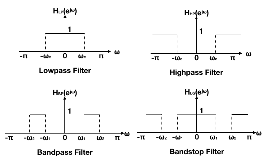
  • 低通濾波器 Lowpass Filter

    使得低頻範圍的訊號通過,抑制高頻範圍的訊號,頻率的閥值稱為截止頻率(Cutoff Frequency) ,定義為 \(f_c\),對應的截止角頻率 \(ω_c\)

  • 高通濾波器 Highpass Filter

    低通濾波器的相反,讓高頻範圍訊號通過,抑制低頻訊號

  • 帶通濾波器 Bandpass Filter

    讓頻率介於 \(f_1 ~ f_2\) 或角頻率 \(ω_1~ω_2\) 之間的訊號通過,抑制其他頻率範圍的訊號

  • 帶阻濾波器 Bandstop Filter

    帶通濾波器的相反,抑制頻率範圍落在 \(f_1 ~ f_2\) 或角頻率 \(ω_1~ω_2\) 之間的訊號,使得其他頻率範圍的訊號通過

  • 陷波濾波器 Notch Filter

    是帶阻濾波器的一種,僅抑制某個特定頻率,ex: 60Hz 的干擾雜訊。陷波濾波器主要是使得某特定頻率的訊號變為 0,因此也稱為歸零濾波器 Nulling Filter

  • 梳狀濾波器 Comb Filter

    Comb Filter 其頻率響應的形狀跟梳子一樣,主要是同時抑制多個頻率範圍,頻率與頻率之間,通常是設定為整數倍數

  • 全通濾波器 All-Pass Filter

    讓所有頻率範圍都通過,通常會調整訊號在某些頻率範圍的相位移

濾波器也可根據訊號的型態分成 類比濾波器 Analog Filter,與數位濾波器 Digital Filter

頻率響應範例

介紹幾種經典的頻率響應

理想濾波器

濾波器的用途是讓某些特定範圍的頻率分量通過,抑制其他範圍的頻率分量,為了不造成訊號失真,頻率通過的頻率分量的頻率響應值是設定為 1,抑制的頻率分量,頻率響應值設定為 0。

使得頻率分量通過的頻率範圍稱為通過頻帶 (Passband),抑制的頻率範圍稱為截止頻帶 (Stopband)

  • 理想低通濾波器 Ideal Lowpass Filter

    轉換函式:\( H_{LP}(e^{jω}) = \left\{ \begin{array}{ll} 1 & \mbox{if 0 ≤ ω ≤ \)ω_c\(} \\ 0 & \mbox{otherwise} \end{array} \right.\)

    在此只定義單邊 Single-Sided 的頻率響應,ω 介於 0 ~ π 之間,且 \(ω_c=2 \pi f_c\),其中 \(f_c\) 稱為截止頻率 Cutoff Frequency

  • 理想高通濾波器 Ideal Highpass Filter

    轉換函式:\( H_{HP}(e^{jω}) = \left\{ \begin{array}{ll} 1 & \mbox{if \)ω_c\( < ω ≤ π} \\ 0 & \mbox{otherwise} \end{array} \right.\)

    低通與高通濾波器的關係為: \(H_{HP}(e^{jω})=1- H_{LP}(e^{jω})\)

  • 理想帶通濾波器 Ideal Bandpass Filter

    轉換函式:\( H_{BP}(e^{jω}) = \left\{ \begin{array}{ll} 1 & \mbox{if \)ω1\( ≤ ω ≤ \)ω2\(} \\ 0 & \mbox{otherwise} \end{array} \right.\)

    允許頻率範圍 \(ω_1 ≤ ω ≤ ω_2\) 或頻率 \(f_1 ≤ f ≤ f_2\) 的訊號通過,\(f_1, f_2\) 稱為截止頻率

  • 理想帶阻濾波器 Ideal Bandstop Filter

    轉換函式:\( H_{BS}(e^{jω}) = \left\{ \begin{array}{ll} 1 & \mbox{if ω < \)ω1\( or ω > \)ω2\(} \\ 0 & \mbox{otherwise} \end{array} \right.\)

    帶通與帶阻濾波器的關係為: \(H_{BS}(e^{jω})=1- H_{BP}(e^{jω})\)


ex: Ideal Lowpass Filter定義如下,求其在離散時間域的脈衝響應 Impulse Response

​ \( H_{LP}(e^{jω}) = \left\{ \begin{array}{ll} ​ 1 & \mbox{if 0 ≤ ω ≤ \)ω_c\(} \\ ​ 0 & \mbox{otherwise} ​ \end{array} \right.\)

根據 Inverse DTFT 公式

\(x[n] = \frac{1}{2π} \int_{-∞}^{∞}X(e^{jωn})e^{jωn}dω\)

Ideal Lowpass Filter 在離散時間域的脈衝響應為:

\(h_{LP}[n] = \frac{1}{2π} \int_{-∞}^{∞}H_{LP}(e^{jωn})e^{jωn}dω \\ = \frac{1}{2π} \int_{-ω_c}^{ω_c}e^{jωn}dω \\ = \frac{1}{2π} [\frac{1}{jn}e^{jωn}]_{-ω_c}^{ω_c} \\ = \frac{1}{2π} [\frac{e^{jω_cn}}{jn}- \frac{e^{-jω_cn}}{jn} ] \\ = \frac{sin(ω_cn)}{πn} \quad\quad \mbox{-∞<n<∞}\)

當 n=0,使用羅必達規則 L'Hopital's Rule

\(h_{LP}[0] = \lim_{n→0} \frac{sin(ω_cn)}{πn} \\ = \lim_{n→0} \frac{ \frac{d}{dn} sin(ω_cn)}{ \frac{d}{dn} (πn) } \\ = \lim_{n→0} \frac{ cos(ω_cn) \cdot ω_c}{ π } \\ = \frac{ ω_c }{ π }\)

因為 \(-∞ < n < ∞\),無法在離散時間域中,定義有限長度的脈衝響應,藉以實現頻率域中的 ideal lowpass filter。脈衝響應在計算時有用到過去、現在、未來的數位訊號,不是因果系統。脈衝響應不符合絕對可加總 Absolutely Summable 原則,系統也不具 BIBO 穩定性。

用 python 處理離散時間域的脈衝響應時,因為離散序列是有限長度,以近似方式接近 ideal lowpass filter。原則上採用的濾波器大小,是使用奇數

當 filter 大小為 5時,-2<n<2

當 filter 大小為 11 時,-5<n<5

ideal lowpass filter 的脈衝響應,具有 sinc 函數的特性,向左右兩邊無限延伸

以下範例選擇 \(ω_c=\frac{\pi}{2}\),因此當 n=0,\(\frac{ω_c}{\pi}=0.5\) ,可調整 \(ω_c\) 觀察脈衝響應的結果

import numpy as np
import matplotlib.pyplot as plt

def plot(filter_size, plotpos):
    filter_half = int( filter_size / 2 )
    wc = np.pi / 2

    na = np.arange( -filter_half, filter_half + 1 ) # 定義 n 陣列
    h = np.zeros( filter_size )                     # 計算脈衝響應
    for n in na:
        if n == 0:
            h[n+filter_half] =  wc/np.pi
        else:
            h[n+filter_half] = np.sin( wc * n ) / ( np.pi * n )

    plt.subplot(plotpos)
    plt.stem( na, h, use_line_collection=True )
    plt.xlabel( 'n (filter_size='+ str(filter_size) +')')
    plt.ylabel( 'h[n]' )

plot(5, 221)
plot(11, 222)
plot(21, 223)
plot(31, 224)

plt.show( )

以下選擇 \(ω_c=\frac{\pi}{10}\),因此當 n=0,\(\frac{ω_c}{\pi}=1/10\)


由於有限長度的脈衝響應,無法提供 ideal filter 的操作特性,在 DSP 實際應用時,通常是讓頻率響應在通過頻帶與截止頻帶之間,由 1 逐漸降為 0,且在通過頻帶或截止頻帶內,頻率響應允許有些微變動。

剛剛是求濾波器大小 5, 11,21, 31 的脈衝響應,現在改求頻率響應。

import numpy as np
import scipy.signal as signal
import matplotlib.pyplot as plt


def plot(filter_size, plotpos):
    filter_half = int( filter_size / 2 )
    wc = np.pi / 2

    na = np.arange( -filter_half, filter_half + 1 ) # 定義 n 陣列
    h = np.zeros( filter_size )                     # 計算脈衝響應
    for n in na:
        if n == 0:
            h[n+filter_half] =  wc/np.pi
        else:
            h[n+filter_half] = np.sin( wc * n ) / ( np.pi * n )

    w, H = signal.freqz( h )
    mag = abs( H )

    plt.subplot(plotpos)
    plt.plot( w, mag )
    plt.xlabel( r'$\omega$'+' (filter_size='+ str(filter_size) +')' )
    plt.ylabel( 'Magnitude' )


plot(5, 221)
plot(11, 222)
plot(21, 223)
plot(31, 224)

plt.show( )

結果發現,若 filter size 越大,或脈衝響應樣本越多,越接近理想的 lowpass filter。此外可注意到頻率響應在通過頻帶與截止頻帶之間,出現了 Gibbs 現象。

平均濾波器

average filter 定義為

\(h[n] = \frac{1}{M}{1,1,1,...,1}, n=0,1,...,M-1\) ,M為濾波器大小 filter size

平均濾波器的頻率響應,可根據其 DTFT 得來

\(H(e^{jω}) = \sum_{n=-∞}^{∞}h[n]e^{-jωn} \\ = \frac{1}{M} \sum_{n=0}^{M-1}e^{-jωn} \\ = \frac{1}{M} ( \sum_{n=0}^{∞}e^{-jωn} - \sum_{n=M}^{∞}e^{-jωn}) \\ = \frac{1}{M} ( \sum_{n=0}^{∞}e^{-jωn} ) (1 - e^{-jωM}) \\ = \frac{1}{M} \frac{1 - e^{-jωM}}{1 - e^{-jω}} \\ = \frac{1}{M} \frac{sin(Mω/2)}{sin(ω/2)} e^{-j(M-1)ω/2} \)

取其強度 magnitude

\(|H(e^{jω})| = |\frac{sin(Mω/2)}{sin(ω/2)}|\)

以圖形表示,就是平均濾波器的頻率響應


ex: 若平均濾波器定義 \(h[n]=\frac{1}{M}{1,1,...,1}, n=0,1,...,M-1\)

當 M=5, 15,求其頻率響應

import numpy as np
import scipy.signal as signal
import matplotlib.pyplot as plt

def average_filter(filter_size):
    h = np.ones( filter_size ) / filter_size
    return h

def plot(filter_size, plotpos):
    h = average_filter(filter_size)

    w, H = signal.freqz( h )
    mag = abs( H )

    plt.subplot(plotpos)
    plt.plot( w, mag )
    plt.xlabel( r'$\omega$'+' (filter_size='+ str(filter_size) +')' )
    plt.ylabel( 'Magnitude' )

plot(5, 121)
plot(15, 122)

plt.show( )

平均濾波器有 lowpass filter 的特性,當 size 越小,通過頻帶越寬。但平均濾波器有允許少量高頻分量通過

高斯濾波器

Gaussian Filter 可定義為

\(g[n]=e^{-n^2/2σ^2}\) ,其中 σ 為標準差

chap9: 高斯函數的傅立葉轉換,形成另一個高斯函數。因此高斯函數的頻率響應,可用另一個高斯函數表示

ex: Gaussian Filter 定義為 \(g[n]=e^{-n^2/2σ^2}\) ,當 σ=1, 3,求其頻率響應

note: 程式中有對係數進行正規化,讓 \(\sum_{n}g[n]=1\)

import numpy as np
import scipy.signal as signal
import matplotlib.pyplot as plt

def plot(sigma, plotpos):
    filter_size = int( 6 * sigma + 1 )              # 濾波器大小
    gauss = signal.gaussian( filter_size, sigma )   # 濾波器係數
    sum = np.sum( gauss )                           # 正規化
    gauss = gauss / sum

    w, H = signal.freqz( gauss )
    mag = abs( H )

    plt.subplot(plotpos)
    plt.plot( w, mag )
    plt.xlabel( r'$\omega$'+' (sigma='+ str(sigma) +')' )
    plt.ylabel( 'Magnitude' )

plot(sigma=1, plotpos=121)
plot(sigma=3, plotpos=122)

plt.show( )

高斯濾波器有 lowpass filter 的特性,標準差越小,通過頻帶較寬。在高頻範圍的抑制效果,比平均濾波器好。

FIR 濾波器

一階 FIR 濾波器有 lowpass, highpass filter 兩種

FIR filters 裡面最簡單的是移動平均濾波器 Moving Averge Filter,濾波器大小為 2

最簡單的 FIR Lowpass Filter 的一階轉換函式定義為:

\(H_0(z)=\frac{1}{2}(1+z^{-1})\)

最簡單的 FIR Highpass Filter 的一階轉換函式定義為:

\(H_1(z)=\frac{1}{2}(1-z^{-1})\)

因為 \(H_1(z) = 1 - H_0(z) = 1-\frac{1}{2}(1+z^{-1}) = \frac{1}{2}(1-z^{-1})\)

ex: 分別求上面兩個 FIR filters 的頻率響應

import numpy as np
import scipy.signal as signal
import matplotlib.pyplot as plt

b = np.array( [ 0.5, 0.5 ] )    # 低通濾波器
w, H0 = signal.freqz( b )
H0 = abs( H0 )

b = np.array( [ 0.5, -0.5 ] )   # 高通濾波器
w, H1 = signal.freqz( b )
H1 = abs( H1 )

plt.subplot(121)
plt.plot( w, H0 )
plt.xlabel( r'$\omega$' +' (lowpass)' )
plt.ylabel( 'Magnitude' )

plt.subplot(122)
plt.plot( w, H1 )
plt.xlabel( r'$\omega$' +' (highpass)' )
plt.ylabel( 'Magnitude' )

plt.show( )
根據 Lowpass Filter 的頻率響應,強度的最大/最小值分別是 1 與 0。頻率響應也是從 1 逐漸降到 0。

在討論 Lowpass Filter 時,當截止頻率 \(ω=ω_0\),強度降為

\(|H_0(e^{jω_c})| = \frac{1}{\sqrt{2}}|H_0(e^{j0})|\)

如果以分貝表示則為

\(20 log_{10}|H_0(e^{jω_c})| = 20 log_{10}( \frac{1}{\sqrt{2}}|H_0(e^{j0})| ) \\ = 20 log_{10}|H_0(e^{j0})| - 20 log_{10}\sqrt{2} \\ = 0 - 3.0103 ≈ -3dB\)

\(ω_c\)或 \(f_c\) 稱為 3dB 截止頻率 (3dB Cutoff Frequency),通常被視為是通過頻帶 (Passband) 的邊緣。因此,\(ω_c\)或 \(f_c\) 也常被稱為 通過頻帶邊緣頻率(Passband Edge Frequency)


串接多個 FIR Filter,可用來近似 ideal lowpass filter

import numpy as np
import scipy.signal as signal
import matplotlib.pyplot as plt

# order = eval( input( "Enter number of cascade FIR filters: " ) )

def plot(order, plotpos):
    b = np.array( [ 0.5, 0.5 ] )
    w, H = signal.freqz( b )

    for i in range( order - 1 ):
        H *= H

    H0 = abs( H )

    plt.subplot(plotpos)
    plt.plot( w, H0 )
    plt.xlabel( r'$\omega$' +'(order='+str(order)+')' )
    plt.ylabel( 'Magnitude' )

plot(1, 221)
plot(2, 222)
plot(3, 223)
plot(4, 224)

plt.show( )

IIR 濾波器

  • IIR Lowpass Filter

    一階 IIR Lowpass Filter 轉換函式定義為 \(H_0(z)= \frac{1-α}{2} \frac{1+z^{-1}}{1-αz^{-1}}\) ,其中 \(|α|<1\) 為穩定的 IIR Filter

  • IIR Highpass Filter

    一階 IIR Highpass Filter 轉換函式定義為 \(H_1(z)= \frac{1+α}{2} \frac{1-z^{-1}}{1-αz^{-1}}\) ,其中 \(|α|<1\) 為穩定的 IIR Filter

ex: 一階 IIR Lowpass/Highpass Filter,當 α = 0.2, 0.4, 0.6, 0.8 時,求其頻率響應

import numpy as np
import scipy.signal as signal
import matplotlib.pyplot as plt

# alpha = eval( input( "Please enter alpha (< 1): " ) )

def iir_lowpass(alpha, plotpos):
    b = np.array( [ 1 - alpha, 1 - alpha ] )
    a = np.array( [ 2, -2 * alpha ] )
    w, H = signal.freqz( b, a )
    H0 = abs( H )

    plt.subplot(plotpos)
    plt.plot( w, H0 )
    plt.xlabel( r'$\omega$' +' (alpha='+str(alpha)+')' )
    plt.ylabel( 'Magnitude' )

def iir_highpass(alpha, plotpos):
    b = np.array( [ 1 + alpha, - ( 1 + alpha ) ] )
    a = np.array( [ 2, -2 * alpha ] )
    w, H = signal.freqz( b, a )
    H1 = abs( H )

    plt.subplot(plotpos)
    plt.plot( w, H1 )
    plt.xlabel( r'$\omega$' +' (alpha='+str(alpha)+')' )
    plt.ylabel( 'Magnitude' )

plt.figure( 1 )
iir_lowpass(0.2, 221)
iir_lowpass(0.4, 222)
iir_lowpass(0.6, 223)
iir_lowpass(0.8, 224)

plt.figure( 2 )
iir_highpass(0.2, 221)
iir_highpass(0.4, 222)
iir_highpass(0.6, 223)
iir_highpass(0.8, 224)

plt.show( )

IIR Lowpass Filters

IIR Highpass Filters

  • IIR 帶通濾波器

    二階 IIR Bandpass Filter 的轉換函式定義為

    \(H_{BP}(z) = \frac{1-α}{2} \frac{1-z^{-2}}{1-β(1+α)z^{-1}+αz^{-2}}\) ,其中 α, β 都小於 1

ex1: 當 α = 0.2, 0.5, 0.8 且 β=0.5 時,求其頻率響應

ex2: 當 α = 0.5 且 β=0.2, 0.5, 0.8 時,求其頻率響應

import numpy as np
import scipy.signal as signal
import matplotlib.pyplot as plt

def IIR_bandpass_frequency_response(alpha, beta, plotpos):
    b = np.array( [ 1 - alpha, 0, -( 1 - alpha ) ] )
    a = np.array( [ 2, -2 * beta * ( 1 + alpha ), 2 * alpha ] )
    w, H = signal.freqz( b, a )
    H1 = abs( H )

    plt.subplot(plotpos)

    plt.plot( w, H1, '-', label = r'$\alpha$ = '+str(alpha)+','+r'$\beta$ = '+str(beta) )
    plt.legend( loc = 'upper right' )
    plt.xlabel( r'$\omega$' )
    plt.ylabel( 'Magnitude' )


IIR_bandpass_frequency_response(0.2, 0.5, 121)
IIR_bandpass_frequency_response(0.5, 0.5, 121)
IIR_bandpass_frequency_response(0.8, 0.5, 121)

IIR_bandpass_frequency_response(0.5, 0.2, 122)
IIR_bandpass_frequency_response(0.5, 0.5, 122)
IIR_bandpass_frequency_response(0.5, 0.8, 122)

plt.show( )

α 參數用來調整頻寬,β 參數用來調整頻率中心

梳狀濾波器

  • Comb Lowpass Filter

    簡易梳狀低通濾波器的轉換函式,可定義為

    \(H_{CLP}(z) = \frac{1}{2}(1+z^{-M})\),M 為正整數

  • Comb Highpass Filter

    簡易梳狀高通濾波器的轉換函式,可定義為

    \(H_{CHP}(z) = \frac{1}{2}(1-z^{-M})\) ,M 為正整數

ex: 當 M=10,求頻率響應

import numpy as np
import scipy.signal as signal
import matplotlib.pyplot as plt

# M = eval( input( "Please enter M for the Comb Filter: " ) )

def comb_lowpass_filter_frequency_response(M, plotpos):

    b = np.zeros( M + 1 )           # 梳狀低通濾波器
    b[0] = 0.5
    b[M] = 0.5
    w, H = signal.freqz( b, 1 )
    H0 = abs( H )

    plt.subplot(plotpos)
    plt.plot( w, H0 )
    plt.xlabel( r'$\omega$'+' (comb lowpass)' )
    plt.ylabel( 'Magnitude' )

def comb_highpass_filter_frequency_response(M, plotpos):

    b = np.zeros( M + 1 )
    b[0] = 0.5
    b[M] = -0.5                     # 梳狀高通濾波器
    w, H = signal.freqz( b, 1 )
    H1 = abs( H )

    plt.subplot(plotpos)
    plt.plot( w, H1 )
    plt.xlabel( r'$\omega$'+' (comb highpass)' )
    plt.ylabel( 'Magnitude' )

M = 10
comb_lowpass_filter_frequency_response(M, 121)
comb_highpass_filter_frequency_response(M, 122)

plt.show( )

References

數位訊號處理:Python程式實作(附範例光碟)(第二版)

2021/2/1

頻譜分析

頻譜分析 spectrum analysis 目的是分析訊號在不同頻率下的分量,以圖形表示。頻譜分析的方法可分成兩大類型:傅立葉頻譜 Fourier Spectrum 與 功率頻密度 Power Spectral Density (PSD)

根據傅立葉基本理論:「任意週期性函數,均可表示成不同頻率、不同振幅的正弦函數或餘弦函數,加總而得的無窮級數。」更進一步,傅立葉轉換也可適用於非週期性函數。

頻譜分析 spectrum analysis 的目的是將訊號分解成不同頻率的分量,並以圖形表示,稱為頻譜(spectrum)。頻譜可用來分析訊號中的頻率分量,例如男生的語音聲音低沈,屬於低頻,女生或兒童是高頻,可藉此辨識說話者是男生、女生或兒童。

弦波的定義為

\(x(t)=A cos(ω_0+ϕ)\) 或是 \(x(t)=A cos(2 \pi f_0t+ϕ)\) ,其中振幅 A ,角頻率 \(ω_0\),頻率 \(f_0\)

根據反尤拉公式 \(cosθ = \frac{e^{jθ}+e^{-jθ}}{2}\)

代入可得

\(x(t) = A cos(ω_0t+ϕ) = A [e^{j(ω_0t+ϕ)}+e^{-j(ω_0t+ϕ)}]/2 \)

因此弦波包含了兩個振幅 Amplitude 的分量,當頻率為 \(ω_0, -ω_0\),振幅均為 A/2,如果以圖形表示,就稱為振幅頻譜 Amplitude Spectrum。

同時弦波 x(t) 也包含了兩個相位移 Phase Shift 的分相,當頻率為 \(ω_0, -ω_0\),相位移分別為 \(ϕ, -ϕ\),如果以圖形表示,稱為相位頻譜 Phase Spectrum。

振幅頻譜及相位頻譜,通稱為傅立葉頻譜 Fourier Spectrum 或頻率頻譜 Frequency Spectrum,或簡稱 Spectrum

由於頻譜是以原點為中心分成兩邊,經常稱為雙邊頻譜 Doubl-Sided Spectrum。頻譜的橫軸以角頻率 ω為主,通常介於 -π ~ π 之間,單位為 弧度/秒 (Raidans/Second),此外,頻譜的橫軸也經常以頻率 f 為主,單位為 Hz

若諧波由多個弦波組成,頻率為基礎頻率的整數倍數,定義為

\(x(t)=\sum_{k=1}^{N}A_k cos(2 \pi f_kt)\),其中 \(f_k=k \cdot f_1\),\(f_1\) 稱為基礎頻率

用反尤拉公式展開後得到振幅頻譜。對應不同頻率的分量,其頻率分量是弦波振幅的一半。

傅立葉頻譜

Fourier Spectrum 是指時間域訊號在頻率域的圖形表示法,可使用傅立葉轉換得來

先對輸入的數位訊號 \(x[n], n=0,1,...,N-1\) 進行離散傅立葉轉換

\(X[k]=\sum_{n=0}^{N-1}x[n]e^{-j2 \pi kn/N}, k=0,1,...,N-1\)

輸出結果為 X[k],是複數構成的離散數列。在 DSP 通常採用 Fast Fourier Transform (FFT) 縮短離散副業轉換的計算所需的時間

FFT 結果為複數,強度為 \(|X[k|, k=0,1,...,N-1\),以圖形表示,稱為強度頻譜 Magnitude Spectrum,也就是前述的振幅頻譜 Amplitude Spectrum。

若求複數的幅角 Argument 或相位角 Phase Angle,並以圖形表示,則稱為相位頻譜 Phase Spectrum

\(arg(X[k]), k=0,1,...,N-1\)


ex: 數位訊號 \(x={1,2,4,3}, n=0,1,2,3\) ,求強度頻譜的圖形

離散傅立葉轉換結果為複數

\(X=\{10, -3+j, 0, -3-j\}\)

強度為 \(|X[0]|=10, |X[1]|=\sqrt{(-3)^2+1^2}=\sqrt{10}\)

Magnitude Spectrum:

弦波

定義 \(x(t)=cos(2 \pi 100 \cdot t)\),振幅 A=1,頻率 f=100,相位移 ϕ=0,在 t=0~1s 之間取 1000 個樣本,取樣頻率 1000Hz,求弦波的傅立葉頻譜?

這邊先以強度頻譜為主,先不討論相位頻譜。由圖形結果可發現 Fourier Spectrum 在 k=100, 900 兩處出現峰值 peaks,形成 Double-Sided Spectrum 的對稱結構,但不是以原點為中心,其中 k=100 的峰值就是弦波的頻率,振幅為 \((A/2) \cdot N = 500\)

為方便傅立葉頻譜的觀察與分析,通常會對 FFT 的結果進行平移 shift,讓頻譜的中心為原點。numpy 的 fftshift 有實現平移的功能。因為 N=1000,根據 Nyquist Theorem,可分析的最大頻率為 500 Hz

import numpy as np
from numpy.fft import fft, fftshift, fftfreq
import matplotlib.pyplot as plt

# time,1000 個 sample 點
t = np.linspace( 0, 1, 1000, endpoint = False )
# 弦波 原始訊號
x = np.cos( 2 * np.pi * 100 * t )

## fft 計算
X = fft( ( x ) )
# 強度
Xm = abs( X )

# 強度頻譜
plt.subplot(121)
plt.plot( Xm )
plt.xlabel( 'k' )
plt.ylabel( 'Magnitude' )

# t = np.linspace( 0, 1, 1000, endpoint = False )
# x = np.cos( 2 * np.pi * 100 * t )

# numpy.fft.fftfreq(n, d=1.0) 定義 Fourier Spectrum 的取樣頻率
# n 為樣本數, d 為取樣週期 (1 second)
# fftshift 用來平移,以原點為中心
f = fftshift( fftfreq( 1000, 0.001 ) )
X = fftshift( fft( x ) )
Xm = abs( X )

plt.subplot(122)
plt.plot( f, Xm )
plt.xlabel( 'f' )
plt.ylabel( 'Magnitude' )

plt.show( )

方波

若方波的參數為 A=1, f=10Hz,在一秒內震盪 10 次,若取樣頻率為 1000Hz,求方波的 Fourier Spectrum ?

方波由無限多個弦波加總而成,可視為一種諧波,基礎頻率為 10Hz,也就是方波的頻率

import numpy as np
import scipy.signal as signal
from numpy.fft import fft, fftshift, fftfreq
import matplotlib.pyplot as plt

# time,1000 個 sample 點
t = np.linspace( 0, 1, 1000, endpoint = False )
# 方波 原始訊號
x = signal.square( 2 * np.pi * 10 * t )

# numpy.fft.fftfreq(n, d=1.0) 定義 Fourier Spectrum 的取樣頻率
# n 為樣本數, d 為取樣週期 (1 second)
# fftshift 用來平移,以原點為中心
f = fftshift( fftfreq( 1000, 0.001 ) )
X = fftshift( fft( x ) )
Xm = abs( X )

plt.plot( f, Xm )
plt.xlabel( 'f' )
plt.ylabel( 'Magnitude' )

plt.show( )

節拍波

beat wave是由兩個不同頻率的弦波乘法運算得來

\(x(t)= A \cdot cos(2 \pi f_1 \cdot t) \cdot cos(2 \pi f_2 \cdot t)\)

通常 \(f_1\) 為低頻訊號的頻率。\(f_2\) 是高頻訊號的頻率,稱為載波頻率 carrier frequency,也常表示為 \(f_c\)。乘法運算是調變 modulation 的主軸,常被用在 DSP 系統中

ex: 節拍波定義為

\(x(t)= \cdot cos(2 \pi 20 \cdot t) \cdot cos(2 \pi 200 \cdot t)\),其中 A=1,\(f_1=20Hz, f_2=200Hz\),取樣頻率為 1000Hz,求 Fourier Spectrum?

import numpy as np
import scipy.signal as signal
from numpy.fft import fft, fftshift, fftfreq
import matplotlib.pyplot as plt

f1 = 20
f2 = 200
t = np.linspace( 0, 1, 1000, endpoint = False )
# 節拍波 原始訊號
x = np.cos( 2 * np.pi * f1 * t ) * np.cos( 2 * np.pi * f2 * t )

f = fftshift( fftfreq( 1000, 0.001 ) )
X = fftshift( fft( x ) )
Xm = abs( X )

plt.plot( f, Xm )
plt.xlabel( 'f' )
plt.ylabel( 'Magnitude' )

plt.show( )

啁啾訊號

這是非週期性訊號

ex: 啁啾訊號在時間 0~1s 之間,頻率範圍是 0Hz 線性遞增到 100Hz,取樣頻率 1000Hz,求 Fourier Spectrum?

頻譜呈現 ripple 現象

import numpy as np
import scipy.signal as signal
from numpy.fft import fft, fftshift, fftfreq
import matplotlib.pyplot as plt

t = np.linspace( 0, 1, 1000, endpoint = False )
x = signal.chirp( t, 0, 1, 100, 'linear' )

f = fftshift( fftfreq( 1000, 0.001 ) )
X = fftshift( fft( x ) ) 
Xm = abs( X )  

plt.plot( f, Xm )
plt.xlabel( 'f' )
plt.ylabel( 'Magnitude' )

plt.show( )

功率頻密度 Power Spectral Density (PSD)

數位訊號的能量 Energy 可定義為

\(E=\int_{-∞}^{∞}|x(t)|^2 {\rm d} t\)

但只適合用來描述有限的訊號。當訊號能量集中在有限時間區間時,總能量有限,因此可透過積分計算而得。

以離散時間域來說,數位訊號的能量可用以下公式計算:

\(E=\sum_{-∞}^{∞}x^2[n]\)


帕塞瓦爾定理

若訊號 \(x(t)\) 的傅立葉轉換為 \(X(f)\),也就是 \(X(f)=\int_{-∞}^{∞}x(t)e^{-j(2 \pi ft)} {\rm d}t\)

則訊號的能量滿足以下公式:

\(E=\int_{-∞}^{∞}|x(t)|^2 {\rm d}t = \int_{-∞}^{∞}|X(f)|^2 {\rm d}f\)

「時間域訊號,若取平方總和(或積分),則結果與傅立葉轉換後頻率域訊號的平方總和(或積分)相等」

換句話說,如果想分析訊號的能量,除了在時間域進行積分外,也可以在頻率域進行積分,結果一樣。

證明:

根據反傅立葉轉換

\(x(t)=\frac{1}{2\pi}\int_{-∞}^{∞}X(ω)e^{jωt} {\rm d}ω\)

則 \(E = \int_{-∞}^{∞} x(t)[\frac{1}{2\pi} \int_{-∞}^{∞}X(ω) e^{jωt} {\rm d}ω ] {\rm d}t \\ = \frac{1}{2 \pi} \int_{-∞}^{∞}X(ω) [\int_{-∞}^{∞} x(t) e^{jωt} {\rm d}t]{\rm d}ω \\ = \frac{1}{2 \pi} \int_{-∞}^{∞}X(ω) X(-ω){\rm d}ω \\ = \frac{1}{2 \pi} \int_{-∞}^{∞}X(ω) X^*(ω){\rm d}ω \quad\quad X^*(ω) 是 X(ω) 的共軛複數 \\ = \frac{1}{2 \pi} \int_{-∞}^{∞} |X(ω)|^2 {\rm d}ω \\ = \frac{1}{2 \pi} \int_{-∞}^{∞} |X(f)|^2 {\rm d}f\)


能量譜密度

若類比訊號 x(t) 的傅立葉轉換為 X(f),則能量譜密度 (Energy Spectral Density) 定義為:

\(X_{xx}(f) = |X(f)|^2\)

能量譜密度的目的是用來描述訊號在不同頻率下的能量分佈狀況,以圖形表示

能量譜密度可根據 自相關 Autocorrelation 取其傅立葉轉換得來

假設訊號 x(t) 的自相關定義為

\(R(τ)=\int_{-∞}^{∞}x^*(t) \cdot x(t+τ) {\rm d}t\)

則其傅立葉轉換為:

\(F\{R(τ)\} = \int_{-∞}^{∞}R(τ)e^{-j2 \pi ft} {\rm d}τ \\ = \int_{-∞}^{∞} [\int_{-∞}^{∞} x^*(t) \cdot x(t+τ) {\rm d}t ] e^{-j2 \pi ft} {\rm d}τ \\ = \int_{-∞}^{∞} x^*(t) [\int_{-∞}^{∞} x(t+τ) e^{-j2 \pi ft} {\rm d}τ ] {\rm d}t \quad\quad 假設 \hatτ = t+τ, {\rm d}\hatτ = {\rm d}τ \\ = \int_{-∞}^{∞} x^*(t) [\int_{-∞}^{∞} x(\hatτ) e^{-j2 \pi f \hatτ} \cdot e^{j2 \pi f t} {\rm d}τ ] {\rm d}t \\ = \int_{-∞}^{∞} x^*(t) [\int_{-∞}^{∞} x(\hatτ) e^{-j2 \pi f \hatτ} {\rm d}τ ] e^{j2 \pi f t} {\rm d}t \\ = \int_{-∞}^{∞} x^*(t) X(f) e^{j2 \pi f t} {\rm d}t \\ = X(f) \int_{-∞}^{∞} x^*(t) e^{j2 \pi f t} {\rm d}t \\ = X(f) X^*(f) \\ = |X(f)|^2 \\ = S_{xx}(f)\)


功率頻密度

功率頻密度 Power Spectral Density 就是訊號在不同頻率下的功率分佈圖

上面的 能量譜密度 定義,只適用於能量集中在某個時間區間的訊號,例如:脈衝訊號。對於持續存在的連續訊號,或是平穩過程 Stationary Process 的訊號,要改用 功率頻密度 Power Spectral Density (PSD),用來描述訊號在不同頻率下,功率 Power 的分佈狀況

評估 功率頻密度 有兩個具代表性的方法:

  • 週期圖 Periodogram

    週期圖是評估功率頻密度最基本的方法,主要根據傅立葉轉換的結果,取平方得來

  • Welch Method

    由 P. D. Welch 提出,也是基於週期圖的方法,但同時參考 Barlett's Method,牽涉功率的平均值運算,又稱為平均週期圖法 Method of Averaged Periodograms


ex: 若產生時間介於 0~1s 的均勻雜訊,值介於 -1~1 之間,取樣頻率 1000Hz,使用週期圖語 Welch Method 求功率頻密度 PSD

這兩種方法得到的功率頻密度,頻率範圍是 0~500Hz (因為 Nyquist Theorem,上限是 500 Hz),在不同頻率下,均勻雜訊都含有少量功率

若以比較嚴謹的定義,理想的 white noise,其功率頻密度在不同頻率下,應該要為固定常數。因此均勻雜訊,並不完全符合 white noise 的條件

import numpy as np
import numpy.random as random
import scipy.signal as signal
import matplotlib.pyplot as plt

fs = 1000
t = np.linspace( 0, 1, fs, endpoint = False )
# 均勻雜訊
noise = random.uniform( -1, 1, fs )

# 用兩種方法求得 PSD
f1, pxx1 = signal.periodogram( noise, fs )
f2, pxx2 = signal.welch( noise, fs )

plt.subplot(121)
plt.plot( f1, pxx1 )
plt.xlabel( 'frequency (Hz)' )
plt.ylabel( 'PSD' )

plt.subplot(122)
plt.plot( f2, pxx2 )
plt.xlabel( 'frequency (Hz)' )
plt.ylabel( 'PSD' )

plt.show( )


ex: 訊號定義為

\(x(t) = 10 cos(2 \pi 100 t) + 5 cos(2 \pi 200 t) + η(t)\)

其中包含兩個弦波,η(t) 是介於 -1~1 之間的均勻雜訊,取樣頻率 1000 Hz,用 週期圖與 Welch Method 求 PSD

兩種方法呈現的 PSD 都是單邊頻譜 Single-Sided Spectrum,範圍是 0~500 Hz。

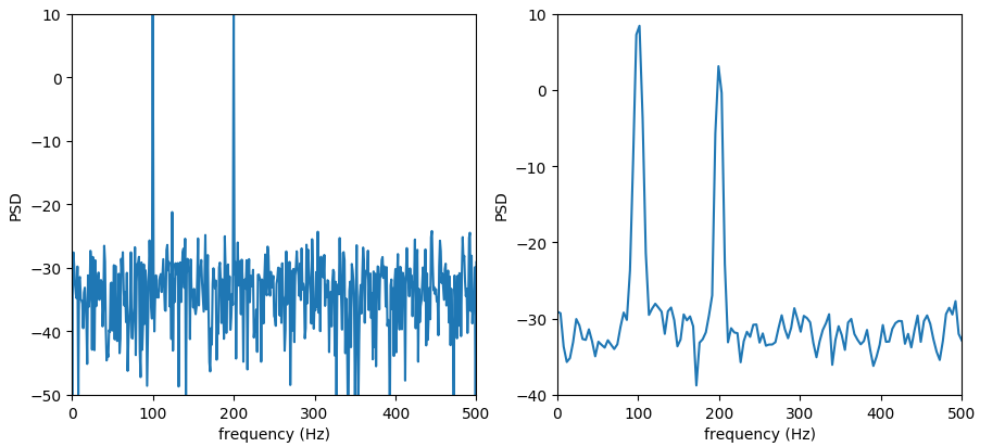
雖然有雜訊干擾, PSD 在 100Hz 與 200Hz 呈現功率的峰值

概括來說,Welch Method 在頻率域上的解析度較差,但具有較好的抗雜訊能力

import numpy as np
import numpy.random as random
import scipy.signal as signal
import matplotlib.pyplot as plt

fs = 1000
t = np.linspace( 0, 1, fs, endpoint = False )
# 原始訊號
x = 10 * np.cos( 2 * np.pi * 100 * t ) + 5 * np.cos( 2 * np.pi * 200 * t ) + random.uniform( -1, 1, fs )

f1, pxx1 = signal.periodogram( x, fs )
f2, pxx2 = signal.welch( x, fs )

plt.subplot(121)
plt.plot( f1, pxx1 )
plt.xlabel( 'frequency (Hz)' )
plt.ylabel( 'PSD' )

plt.subplot(122)
plt.plot( f2, pxx2 )
plt.xlabel( 'frequency (Hz)' )
plt.ylabel( 'PSD' )

plt.show( )

也可再對 PSD 取對數,查看主要頻率外,其他頻率的分佈狀況

import numpy as np
import numpy.random as random
import scipy.signal as signal
import matplotlib.pyplot as plt

fs = 1000
t = np.linspace( 0, 1, fs, endpoint = False )
x = 10 * np.cos( 2 * np.pi * 100 * t ) + 5 * np.cos( 2 * np.pi * 200 * t )
noise = random.uniform( -1, 1, fs )
y = x + noise

f1, pxx1 = signal.periodogram( y, fs )
f2, pxx2 = signal.welch( y, fs )

# 取對數
lp1 = 10 * np.log10( pxx1 )
lp2 = 10 * np.log10( pxx2 )

plt.subplot(121)
plt.plot( f1, lp1 )
plt.xlabel( 'frequency (Hz)' )
plt.ylabel( 'PSD' )
plt.axis( [ 0, 500, -50, 10 ] )

plt.subplot(122)
plt.plot( f2, lp2 )
plt.xlabel( 'frequency (Hz)' )
plt.ylabel( 'PSD' )
plt.axis( [ 0, 500, -40, 10 ] )

plt.show( )

References

數位訊號處理:Python程式實作(附範例光碟)(第二版)