2020/11/16

數位訊號

類比訊號透過取樣 sampling 與量化 quantization 兩個步驟,擷取數位訊號,並以數學表示法討論數位訊號。

數位訊號定義為:隨著時間改變的離散訊號,也稱為離散時間訊號 Discrete-Time Signals

自然界的訊號通常都是類比訊號,因此必須先透過類比/數位轉換器 Analog/Digital Converter, A/D Converter 將類比訊號轉成數位訊號,以便電腦系統處理。過程是根據類比訊號,在時間軸上擷取離散的樣本 samples,藉以產生數位訊號。x(t) 代表類比訊號,x[n] 代表數位訊號,t 為時間,n 是索引。

取樣與量化

取樣 sampling 可定義為 \(x[n]=x(nT_s)\),\(T_s\) 稱為取樣週期 sampling period 或取樣間隔 sampling interval,單位為 second,另外 \(f_s=\frac{1}{T_s}\) 稱為取樣頻率 sampling frequency,或取樣率 sampling rate

取樣是訊號在時間軸上的數位化過程,每隔 \(T_s\) 時間,擷取一個樣本 sample,產生一個數字序列,因每個樣本來自短暫的時間框,也稱為音框 frame

取樣率 sampling frequency 解釋為:每秒取樣的次數。由於取樣頻率固定不變,又稱為均勻取樣 Uniform Sampling

ex: 弦波 \(x(t)=A cos(ωt+ϕ) = Acos(2 \pi ft+ϕ)\) ,若取樣週期 \(T_s\),取樣頻率 \(f_s\),則弦波的數位訊號可表示為

\(x[n]=x(nT_s)=A cos(2 \pi fnT_s+ϕ)=A cos(2 \pi fn/f_s+ϕ)\),n為整數

通常可假設 \(\hat{ω} = 2 \pi f/f_s\) 稱為正規化角頻率 Normalized Angular Frequency,單位是弧度 Radians,因此數位訊號也可表示為

\(x[n] = A cos(\hat{ω}n+ϕ)\)

Nyquist-Shannon 取樣定理

假設原始訊號為頻帶限制訊號 Band-Limited Signal,最高頻率為 \(f_H\),若取樣頻率為 \(f_s\) ,則 \(f_s > 2 f_H\) 時,才能保證可重建原始訊號

若取樣頻率超過原始訊號的最高頻率的兩倍,可充分表示原始訊號,如取樣頻率不足,會產生混疊 aliasing 現象。

ex: 人類聽力範圍 20Hz ~ 20k Hz,最高為 20kHz,如果 \(f_s>40kHz\) 可充分表示人類可感知的原始訊號。目前 mp3 通常設定為 44kHz or 48kHz,符合基本條件,不會發生 aliasing

根據取樣定理,取樣頻率決定了可取樣的原始最高頻率,又稱為 Nyquist 頻率。例如取樣頻率 44kHz,則 Nyquist 頻率為 22kHz

量化 Quantization

量化是將訊號的振幅 Amplitude 經過數位化轉換為數值,常用的數值範圍:

  • 8 bits: 0~255 or -128~127
  • 16 bits: -32768 ~ 32767

每個樣本可使用的位元數稱為位元解析度 bit resolution,或稱為位元深度 bit depth。

數學表示法

\(x=\{x[n]\}, -∞<n<∞\),n 為整數

DSP 系統中,數位訊號通常為有限 finite 數字序列,可表示為

\(x=\{x[n]\}, n=0,1,2..., N-1\) ,這是從 t=0 開始的樣本,N為樣本數

import numpy as np
import matplotlib.pyplot as plt

n = np.array( [ 0, 1, 2, 3, 4, 5 ] )    # 定義n陣列
x = np.array( [ 1, 2, 4, 3, 2, 1 ] )    # 定義x陣列

plt.stem( n, x, use_line_collection=True )                      # 繪圖
plt.xlabel( 'n' )
plt.ylabel( 'x[n]' )
plt.show( )

基本的數位訊號

單位脈衝函數

Unit Impulse Function 也稱為狄拉克 δ 函數 (Dirac Delta Function),以英國物理學家 Paul Dirac 命名,定義:

\(δ(t)=0, t \neq 0\) ,且 \(\int_{-∞}^{∞}δ(t) {\rm d}t = 1\)

單位脈衝函數是連續時間函數,除了原點 t=0 以外,函數值均為 0,在時間域的積分(總面積)為 1,且集中在原點

單位脈衝

在離散時間域的 Unit Impulse 定義為

\( δ[n] = \left\{ \begin{array}{ll} 1, & \mbox{if n=0} \\ 0, & \mbox{if n≠0} \end{array} \right.\)

單位步階函數

Unit Step Function 也稱為黑維塞步階函數 (Heaviside Step Function),以英國科學家 Oliver Heaviside 命名,定義為

\( μ(t) = \left\{ \begin{array}{ll} 1, & \mbox{if t ≥0} \\ 0, & \mbox{if t<0} \end{array} \right.\)

單位步階

Unit Step 定義為

\( μ[n] = \left\{ \begin{array}{ll} 1, & \mbox{if n ≥0} \\ 0, & \mbox{if n<0} \end{array} \right.\)


單位脈衝的時間延遲 Time Delay 定義為 \(δ[n-n_0]\)

ex: \(δ[n-2]\) 的圖形為

因此 Unit Step 也可表示為

\( μ[n] = δ[n]+δ[n-1]+δ[n-2]+... = \sum_{k=0}^{n}δ[n-k]\)

單位脈衝 Unit Impulse 也可表示為

\(δ[n]=μ[n]-μ[n-1]\)

任意數位訊號都可以用單位脈衝表示為

\(x[n]=...+x[-1]δ[n+1]+x[0]δ[n]+x[1]δ[n-1]+... = \sum_{k=-∞}^{∞}x[k]δ[n-k]\)

數位語音檔

波型音訊檔案格式 Waveform Audio File Format、wave,是 Microsoft 與 IBM 制定的音訊編碼格式。另外 Apple Mac 定義了 aiff 音訊格式。

wav 是根據 Resource Interchange File Format(RIFF) ,為了存取 CD 數位音樂而設計的。前面是 header 共44 bytes,內容由多個區塊 chunks 組成,每個區塊是 4 bytes

起始位址(Bytes) 位址範圍 區塊名稱 區塊大小 ( Bytes) 內容 說明
0 1 ~ 4 區塊編號 4 RIFF Marks the file as a riff file.
4 5 ~ 8 總區塊大小 4 N + 36 File size (integer) Size of the overall file - 8 bytes
8 9 ~ 12 檔案格式 4 "WAVE" File Type Header. For our purposes, it always equals "WAVE".
12 13~16 子區塊 1 標籤 4 "fmt " Format chunk marker. Includes trailing null
16 17~20 子區塊 1 大小 4 16 Length of format data as listed above
20 21~22 音訊格式 2 1(PCM) Type of format (1 is PCM)
22 23~24 通道數量 2 1: (mono), 2: stereo Number of Channels
24 25~28 取樣頻率 4 Hz Sample Rate, Common values are 44100 (CD), 48000 (DAT). Sample Rate = Number of Samples per second, or Hertz
28 29~32 位元組 ByteRate 4 ByteRate = (Sample Rate * BitsPerSample * Channels) / 8 取樣頻率 * 位元深度 / 8
32 33~34 區塊對齊 BlockAlign 2 4 (BitsPerSample * Channels) / 8 The number of bytes for one sample including all channels ex: 1 -> 8 bit mono, 2 -> 8 bit stereo/16 bit mono, 4 -> 16 bit stereo
34 35~36 位元深度 2 16 Bits per sample
36 37~40 子區塊2標籤 4 "data" "data" chunk header. Marks the beginning of the data section.
40 41~44 子區塊2大小 4 N Size of the data section, i.e. file size - 44 bytes header.
44 45~ 資料 N 音訊資料

wav 沒有採用壓縮技術,檔案大小比其他格式大,但 wav 不會發生失真的狀況。

import wave

filename = input( "Please enter file name: " )
wav = wave.open( filename, 'rb' )

num_channels = wav.getnchannels( )  # 通道數
sampwidth   = wav.getsampwidth( )   # 樣本寬度
frame_rate  = wav.getframerate( )   # 取樣率
num_frames  = wav.getnframes( )     # 音框數
comptype    = wav.getcomptype( )    # 壓縮型態
compname    = wav.getcompname( )    # 壓縮名稱

print( "Number of Channels =", num_channels )
print( "Sample Width =", sampwidth )
print( "Sampling Rate =", frame_rate )
print( "Number of Frames =", num_frames )
print( "Comptype =", comptype )
print( "Compname =", compname )

wav.close( )

要讀取 wav 的資料,可改用 SciPy 的 io.wavfile 套件,讀取後以 numpy 的陣列回傳

from scipy.io import wavfile
import matplotlib.pyplot as plt

filename = input( "Please enter file name: " )
sampling_rate, x = wavfile.read( filename )

plt.plot( x )
plt.xlabel( 'n' )
plt.ylabel( 'Amplitude' )

plt.show( )

可直接取得 microphone 語音的波形

pip install PyAudio
import numpy as np
import pyaudio
import matplotlib.pyplot as plt

# sampling rate
fs = 11000
# 每次擷取樣本數 1024
CHUNK = 1024
pa = pyaudio.PyAudio( )
stream = pa.open( format = pyaudio.paInt16, channels = 1, rate = fs, 
                  input = True, output = False, frames_per_buffer = CHUNK )
            
try:            
    while True:                     
        data = stream.read( CHUNK )
    # 字串轉換為 int16
        x = np.fromstring( data, np.int16 )

        plt.clf( )
        plt.plot( x )
        plt.axis( [ 0, CHUNK, -30000, 30000 ] )

        plt.pause( 0.1 )

except KeyboardInterrupt:
    print( "Quit" )
    pa.close( stream )
    quit( )

References

數位訊號處理:Python程式實作(附範例光碟)(第二版)

2020/11/9

類比訊號

典型的類比訊號稱為弦波 Sinusoids,弦波的數學模型,可表示成複數指數系統。最後介紹相量 Phasor 的定義,同時討論與證明相量加法規則 Phasor Addition Rule

類比訊號 analog signals 可定義為:隨著時間改變的連續訊號,用函數表示為 \(x=f(t)\),其中 t 為時間,x 是隨著時間改變的連續訊號

弦波 sinusoids

可用餘弦函數定義為 \(x(t)= A cos (ωt+ϕ)\) 或 \(x(t)=A cos(2 \pi ft+ϕ)\)

其中 A 為振幅 Amplitude,ω 為角頻率 Angular Frequency,f 為頻率,ϕ 為相位移 Phase Shift,且 \(ω = 2 \pi f\)

具有週期性 \(T=\frac{1}{f}\)

ω 為角頻率,單位是 弧度/秒 (Radians/Second) ,\(ω = 2 \pi f = \frac{2 \pi}{T}\)

頻率的單位是 次數/秒 (Cycles/Second) 或 Hz

相位移的單位是 弧度 (Radians)

import numpy as np
import matplotlib.pyplot as plt

def sinusoids(amplitude, frequency, phase_shift, plotpos):
    t = np.linspace( 0, 2, 1000, endpoint = False ) # 定義時間陣列
    x = amplitude * np.cos( 2 * np.pi * frequency * t + phase_shift ) # 產生弦波

    plt.subplot(plotpos)
    # plt.ylim(-4,4)

    plt.plot( t, x )                                # 繪圖
    plt.xlabel( 't (second)' )
    plt.ylabel( 'Amplitude' )

# 振幅 = 1, 2, 4
plt.figure( 1 )
# 1*cos(2*pi*2*t)
sinusoids(1, 2, 0, '131')
# 2*cos(2*pi*2*t)
sinusoids(2, 2, 0, '132')
# 4*cos(2*pi*2*t)
sinusoids(4, 2, 0, '133')

# 頻率 = 1,2,4
plt.figure( 2 )
# 1*cos(2*pi*1*t)
sinusoids(1, 1, 0, '131')
# 1*cos(2*pi*2*t)
sinusoids(1, 2, 0, '132')
# 1*cos(2*pi*4*t)
sinusoids(1, 4, 0, '133')


# 相位移 = 0, pi/4, pi/2
plt.figure( 3 )
# 1*cos(2*pi*1*t)
sinusoids(1, 1, 0, '131')
# 1*cos(2*pi*2*t)
sinusoids(1, 1, np.pi/4, '132')
# 1*cos(2*pi*4*t)
sinusoids(1, 1, np.pi/2, '133')

plt.show( )

ex: \(x(t)=Acos(2 \pi ft+ϕ)\)

振幅 A = 1,2,4

頻率 f = 2

相位移 ϕ = 0

結果:當 A 越大,音量越大

ex: \(x(t)=Acos(2 \pi ft+ϕ)\)

振幅 A = 1

頻率 f = 1,2,4

相位移 ϕ = 0

結果:當 f 越大,音頻越高,每秒震盪次數越大

ex: \(x(t)=Acos(2 \pi ft+ϕ)\)

振幅 A = 1

頻率 f = 1

相位移 ϕ = 0, π/4, π/2

結果:弦波會向左移動 0, π/4, π/2,若 ϕ 為負值,則是向右移,稱為時間延遲 (Time Delay)。相位移不會改變波形

複數 complex number

定義為 \(z=a+bj\) ,其中 a 為實部 real part, b 為虛部 imaginary part,\(j=\sqrt{-1}\) 為虛數的單位

  • 複數可用複數平面 complex plane 表示

  • 極座標 Polar Coordinate System 的方式表示

\(z = |z|(cosθ + j sinθ)\) ,其中

\(|z|=\sqrt{a^2+b^2}\),稱為複數的強度 (magnitude)

\(θ = tan^{-1}(b/a)\) ,稱為複數的幅角 (argument) 或相位角 (Phase Angle)

note: arctan 的值域為 \((-\frac{\pi}{2}, \frac{\pi}{2})\),第二、三象限的角度,無法直接用 arctan 計算

  • 根據尤拉公式(Euler's Equation) \(e^{jθ} = cos θ + j sinθ\),複數也可表示為極座標表示法

    \(z=|z|e^{jθ}\)

ex: 複數 \(z=3+4j\) ,求強度 magnitude,相位角 Phase Angle

import numpy as np

# z = - 3 + 4j                          # 定義複數
z = complex(3,4)
magnitude = abs( z )                # 計算強度(Magnitude)
theta = np.angle( z ) * 180 / np.pi # 計算相位角(Phase Angle)

print( "z =", z )
print( "Magnitude =", magnitude )
print( "Phase Angle =", theta )
$ python complex_number.py
z = (3+4j)
Magnitude = 5.0
Phase Angle = 53.13010235415598

強度 magnitude

\(|z|=\sqrt{3^2+4^2} = 5\)

相位角

\(θ = tan^{-1}(4/3) = 52.13^{\circ}\)


複數的運算

  • \(j=\sqrt{-1}, j^2 = -1\)

  • 加法

    \((a+bj)+(c+dj) = (a+c)+(b+d)j\)

  • 減法

    \((a+bj)-(c+dj) = (a-c)+(b-d)j\)

  • 乘法

    \((a+bj)(c+dj) = (ac-bd)+(bc+ad)j\)

  • 除法

    \(\frac{a+bj}{c+dj} = \frac{(a+bj)(c-dj)}{(c+dj)(c-dj)} = \frac{(ac+bd)+(bc-ad)j}{c^2+d^2}\)

  • 反尤拉公式

    \(cosθ = \frac{e^{jθ}+e^{-jθ}}{2}, sinθ= \frac{e^{jθ}-e^{-jθ}}{2j}\)


ex: 用複數證明三角函數的和角公式

\(cos(α+β) = Re\{cos(α+β) + jsin(α+β)\} \\ = Re\{e^{j(α+β)}\} \\ = Re\{e^{jα}+e^{jβ}\} \\ = Re\{(cosα+jsinα) \cdot (cosβ+jsinβ)\} \\ = Re\{(cosα \cdot cosβ - sinα \cdot sinβ) + j (sinα \cdot cosβ+cosα \cdot sinβ)\}\)

因此

\(cos(α+β) = cosα \cdot cosβ - sinα \cdot sinβ\)

\(sin(α+β) = sinα \cdot cosβ+cosα \cdot sinβ\)


複數指數訊號

complex exponential signals 定義為

\(z(t) = A e^{j(ωt+ϕ)}\) ,其中 A 是振幅 amplitude,(ωt+ϕ) 是相位角 Phase Angle

根據弦波定義 \(x(t)=A cos(ωt+ϕ)\) 與尤拉公式 \(e^{jθ} = cosθ+jsinθ\)

\(z(t) = A e^{j(ωt+ϕ)} = A cos(ωt+ϕ)+A \cdot jsin(ωt+ϕ)\)

因此 \(x(t) = Re\{z(t)\}\) 弦波,是複數指數訊號 z(t) 的實部

相量

相量 Phasor 定義為 \(X= A e^{jϕ}\),其中 A 是振幅 amplitude,ϕ 是相位移 phase shift

根據複數指數訊號的定義

\(z(t) = A e^{j(ωt+ϕ)} = Ae^{jωt} \cdot e^{jϕ} = Ae^{jϕ} \cdot e^{jωt}\)

因此定義 \(X=Ae^{jϕ}\),就是 Phasor


ex: 求弦波 \(x(t)=10 cos(2 \pi t+\pi /4)\) 的 phasor

因為 A =10, f=1, ϕ=π/4

phasor = \(Ae^{jϕ} = 10e^{j\pi/4} = 10 \cdot (cos\frac{\pi}{4}+jsin\frac{\pi}{4}) = 5\sqrt{2}+5\sqrt{2}j\)


Phasor 就是複數平面上的向量 vector


ex: 兩個頻率相同的弦波相加的結果,頻率不變

\(x_1(t) = 3 cos(2 \pi 10 t + \pi/4)\)

\(x_2(t) = 4 cos(2 \pi 10 t + 3\pi/4)\)

import numpy as np
import matplotlib.pyplot as plt

t = np.linspace( 0, 1, 1000, endpoint = False )         # 定義時間陣列
x1 = 3 * np.cos( 2 * np.pi * 10 * t + np.pi / 4 )       # 第一個弦波
x2 = 4 * np.cos( 2 * np.pi * 10 * t + 3 * np.pi / 4 )   # 第二個弦波
x3 = x1 + x2                                            # 弦波相加

plt.plot( t, x1, '--', label = 'x1(t)' )                # 繪圖
plt.plot( t, x2, '--', label = 'x2(t)' )
plt.plot( t, x3, '-', label = 'x3(t)' )

plt.legend( loc = 'upper right' )
plt.xlabel( 't (second)' )
plt.ylabel( 'Amplitude' )
plt.axis( [ 0, 1, -6, 6 ] )

plt.show( )

相量加法規則

相量加法規則:有 N 個弦波,角頻率都是 \(ω_0\),振幅與相位移分別為 \(A_k, ϕ_k, k=1,2,...N\),則

\(\sum_{k=1}^{N}A_kcos(ω_0t+ϕ_k) = Acos(ω_0t+ϕ)\)

換句話說,若有 N 個弦波,角頻率 \(ω_0\) (或頻率 \(f_0\)) 都相同,則相加後的弦波,角頻率 (或頻率) 會維持不變

證明:用複數的運算規則

\(\sum_{k=1}^{N}A_kcos(ω_0t+ϕ_k) = \sum_{k=1}^{N}Re\{A_ke^{j(ω_0t+ϕ_k)}\} \\ = Re\{ \sum_{k=1}^{N} A_ke^{j(ω_0t+ϕ_k)}\} \\ = Re\{ \sum_{k=1}^{N} A_ke^{jϕ_k} \cdot e^{jω_0t}\} \\ = Re\{ (\sum_{k=1}^{N} A_ke^{jϕ_k}) \cdot e^{jω_0t}\} \\ = Re\{ Ae^{jϕ} \cdot e^{jω_0t}\} \\ = Re\{ Ae^{j(ω_0t+ϕ)}\} \\ = Acos(ω_0t+ϕ)\)

以上推導過程要滿足 \(\sum_{k=1}^{N} A_ke^{jϕ_k} = Ae^{jϕ} \)

也就是 N 個弦波相加後結果,振幅 A 與 相位移 ϕ ,可根據個弦波的 Phasors,取其總和來決定


ex: 有兩個弦波,計算加總後 \(x_3(t)=x_1(t)+x_2(t)\) 的振幅及相位移

\(x_1(t) = 3 cos(2 \pi 10 t + \pi/4)\)

\(x_2(t) = 4 cos(2 \pi 10 t + 3\pi/4)\)

先計算兩個弦波的 phasors

\(A_1e^{jϕ_1} = 3 e^{j \pi/4} = 3 cos(\frac{\pi}{4}) + j sin(\frac{\pi}{4})\)

\(A_2e^{jϕ_1} = 4 e^{j 3 \pi/4} = 4 cos(\frac{3\pi}{4}) + j sin(\frac{3\pi}{4})\)

相加後的 phasor (複數加法)

\(Ae^{jϕ} = (3 cos(\frac{\pi}{4})+4 cos(\frac{3\pi}{4}) ) + j(sin(\frac{\pi}{4})+sin(\frac{3\pi}{4})) \\ = -\frac{1}{\sqrt{2}} + j \frac{7}{\sqrt{2}}\)

轉換為極座標 \(z = |z| (cosθ+jsinθ)\) \( z=a+bj, |z| = \sqrt{a^2+b^2}, θ = tan^{-1}(b/a)\)

\(A=|z| = 5\)

\(ϕ = \pi - tan^{-1}(7) = 1.7127\) note: 第二象限的 arctan

因此 \(x_3(t) = 5 cos(2 \pi 10 t+1.7127)\)

import numpy as np

phasor1 = complex( 3 * np.cos( np.pi / 4 ), 3 * np.sin( np.pi / 4 ) )
phasor2 = complex( 4 * np.cos( 3 * np.pi / 4 ), 4 * np.sin( 3 * np.pi / 4 ) )
phasor = phasor1 + phasor2

A = abs( phasor )                   
phi = np.angle( phasor ) 

print( "Phasor1 =", phasor1 )
print( "Phasor2 =", phasor2 )
print( "Phasor =", phasor )
print( "Amplitude =", A )
print( "Phase Angle =", phi )

執行結果

Phasor1 = (2.121320343559643+2.1213203435596424j)
Phasor2 = (-2.82842712474619+2.8284271247461903j)
Phasor = (-0.707106781186547+4.949747468305833j)
Amplitude = 5.0
Phase Angle = 1.7126933813990604

References

數位訊號處理:Python程式實作(附範例光碟)(第二版)

2020/11/2

TensorFlow手寫數字辨識_MLP

tensorflow 的 MNIST 資料及共有訓練資料 55000 筆,驗證資料 5000筆,每一筆資料由 feature (影像)與 label (數字) 組成。

注意:要改用 tensorflow.keras.datasets

tensorflow.examples.tutorials is now deprecated and it is recommended to use tensorflow.keras.datasets

MNIST 資料處理

import tensorflow as tf
import numpy as np

mnist = tf.keras.datasets.mnist
# Tuple of Numpy arrays: (x_train, y_train), (x_test, y_test)

(x_train, y_train), (x_test, y_test) = mnist.load_data()
# 將每個 pixel 的值從 Int 轉成 floating point 同時做normalize(這是很常見的preprocessing)
# x_train, x_test = x_train / 255.0, x_test / 255.0

# 查看 train Data
print('x_train length = ', len(x_train), ', x_test length = ', len(x_test))
# x_train length =  60000 , x_test length =  10000
print('x_train.shape = ', x_train.shape, ', x_train[0].shape = ', x_train[0].shape, ', x_test[0].shape=', x_test[0].shape)
# 每張圖片 大小為 28x28
# x_train.shape =  (60000, 28, 28) , x_train[0].shape =  (28, 28) , x_test[0].shape= (28, 28)

print('x_train[0].length = ', len(x_train[0]) )
# x_train[0].length =  28
print('y_train length = ', len(y_train), ', y_train[0] = ', y_train[0])
# y_train length =  60000 , y_train[0] =  5


# 將 第一張 x_train 的圖片儲存到檔案
import matplotlib.pyplot as plt
def plot_image(image, filename):
    plt.clf()
    plt.imshow(image.reshape(28,28), cmap='binary')
    plt.savefig(filename)
plot_image(x_train[0], "x_train_index_0.png")


# 將 training 的 input 資料 28*28 的 2維陣列 轉為 1維陣列,再轉成 float32
# 每一個圖片,都變成 784 個 float 的 array
# training 與 testing 資料數量分別是 60000 與 10000 筆
# X_train_2D 是 [60000, 28*28] 的 2維陣列
x_train_2D = x_train.reshape(60000, 28*28).astype('float32')
x_test_2D = x_test.reshape(10000, 28*28).astype('float32')
print('x_train_2D.shape=', x_train_2D.shape)
# x_train_2D.shape=(60000, 784)


# 將圖片的數字 (0~255) 標準化,最簡單的方法就是直接除以 255
# x_train_norm 是標準化後的結果,每一個數字介於 0~1 之間
x_train_norm = x_train_2D/255
x_test_norm = x_test_2D/255

# 將 training 的 label 進行 one-hot encoding,例如數字 7 經過 One-hot encoding 轉換後是 array([0., 0., 0., 0., 0., 0., 0., 1., 0., 0.], dtype=float32),即第7個值為 1

one_hot=tf.one_hot(y_train,10)

with tf.compat.v1.Session() as sess:
    init = tf.compat.v1.global_variables_initializer()
    sess.run(init)
    y_train_one_hot = sess.run(one_hot)

    print( y_train_one_hot )
    print( 'y_train[0] = ', y_train[0], ", y_train_one_hot[0]=", y_train_one_hot[0] )
    # y_train[0] =  5 , y_train_one_hot[0]= [0. 0. 0. 0. 0. 1. 0. 0. 0. 0.]

    # 也可以用 np.argmax 將 one_hot 陣列,轉換回原本的數字
    print( 'y_train[0] = ', np.argmax(y_train_one_hot[0]) )
    # y_train[0] =  5

    # 列印前10筆 one hot
    for i in range(10):
        print(y_train_one_hot[i])
        # [0. 0. 0. 0. 0. 1. 0. 0. 0. 0.]
        # [1. 0. 0. 0. 0. 0. 0. 0. 0. 0.]
        # [0. 0. 0. 0. 1. 0. 0. 0. 0. 0.]
        # [0. 1. 0. 0. 0. 0. 0. 0. 0. 0.]
        # [0. 0. 0. 0. 0. 0. 0. 0. 0. 1.]
        # [0. 0. 1. 0. 0. 0. 0. 0. 0. 0.]
        # [0. 1. 0. 0. 0. 0. 0. 0. 0. 0.]
        # [0. 0. 0. 1. 0. 0. 0. 0. 0. 0.]
        # [0. 1. 0. 0. 0. 0. 0. 0. 0. 0.]
        # [0. 0. 0. 0. 1. 0. 0. 0. 0. 0.]

用一個 function 列印多筆圖片, label 資訊

import tensorflow as tf
import numpy as np

mnist = tf.keras.datasets.mnist
# Tuple of Numpy arrays: (x_train, y_train), (x_test, y_test)

(x_train, y_train), (x_test, y_test) = mnist.load_data()

# 將 training 的 input 資料 28*28 的 2維陣列 轉為 1維陣列,再轉成 float32
# 每一個圖片,都變成 784 個 float 的 array
# training 與 testing 資料數量分別是 60000 與 10000 筆
# X_train_2D 是 [60000, 28*28] 的 2維陣列
x_train_2D = x_train.reshape(60000, 28*28).astype('float32')
x_test_2D = x_test.reshape(10000, 28*28).astype('float32')
print('x_train_2D.shape=', x_train_2D.shape)
# x_train_2D.shape=(60000, 784)

# 將圖片的數字 (0~255) 標準化,最簡單的方法就是直接除以 255
# x_train_norm 是標準化後的結果,每一個數字介於 0~1 之間
x_train_norm = x_train_2D/255
x_test_norm = x_test_2D/255

# 將 training 的 label 進行 one-hot encoding,例如數字 7 經過 One-hot encoding 轉換後是 array([0., 0., 0., 0., 0., 0., 0., 1., 0., 0.], dtype=float32),即第7個值為 1

y_train_one_hot_tf=tf.one_hot(y_train,10)
y_test_one_hot_tf=tf.one_hot(y_test,10)

with tf.compat.v1.Session() as sess:
    init = tf.compat.v1.global_variables_initializer()
    sess.run(init)
    y_train_one_hot = sess.run(y_train_one_hot_tf)
    y_test_one_hot = sess.run(y_test_one_hot_tf)


# 查看多筆資料,以及 label
import matplotlib.pyplot as plt
def plot_images_labels_prediction(images,labels,prediction,idx,filename, num=10):
    fig = plt.gcf()
    fig.set_size_inches(12, 14)
    if num>25: num=25
    for i in range(0, num):
        ax=plt.subplot(5,5, 1+i)

        # 將 images 的 784 個數字轉換為 28x28
        ax.imshow(np.reshape(images[idx],(28, 28)), cmap='binary')

        # 轉換 one_hot label 為數字
        title= "label=" +str(np.argmax(labels[idx]))
        if len(prediction)>0:
            title+=",predict="+str(prediction[idx])

        ax.set_title(title,fontsize=10)
        ax.set_xticks([]);ax.set_yticks([])
        idx+=1
    plt.savefig(filename)

plot_images_labels_prediction(x_train_2D, y_train_one_hot,[], 0, 'x_train_0.png', 10)
plot_images_labels_prediction(x_train_2D, y_train_one_hot,[], 10, 'x_train_1.png', 10)

plot_images_labels_prediction(x_test_2D, y_test_one_hot,[], 0, 'x_test_0.png', 10)
plot_images_labels_prediction(x_test_2D, y_test_one_hot,[], 10, 'x_test_1.png', 10)

以 tensorflow 建立 MLP

訓練部分資料共有 60000 筆,經過預處理後,會產生 feature, label,然後輸入 MLP model 進行訓練,訓練完成的模型,可在預測階段使用。

import tensorflow as tf
import numpy as np

# STEP 1 讀取資料
mnist = tf.keras.datasets.mnist
# Tuple of Numpy arrays: (x_train, y_train), (x_test, y_test)

(x_train, y_train), (x_test, y_test) = mnist.load_data()

# 將 training 的 input 資料 28*28 的 2維陣列 轉為 1維陣列,再轉成 float32
# 每一個圖片,都變成 784 個 float 的 array
# training 與 testing 資料數量分別是 60000 與 10000 筆
# X_train_2D 是 [60000, 28*28] 的 2維陣列
x_train_2D = x_train.reshape(60000, 28*28).astype('float32')
x_test_2D = x_test.reshape(10000, 28*28).astype('float32')
print('x_train_2D.shape=', x_train_2D.shape)
# x_train_2D.shape=(60000, 784)

# 將圖片的數字 (0~255) 標準化,最簡單的方法就是直接除以 255
# x_train_norm 是標準化後的結果,每一個數字介於 0~1 之間
x_train_norm = x_train_2D/255
x_test_norm = x_test_2D/255

# 將 training 的 label 進行 one-hot encoding,例如數字 7 經過 One-hot encoding 轉換後是 array([0., 0., 0., 0., 0., 0., 0., 1., 0., 0.], dtype=float32),即第7個值為 1

y_train_one_hot_tf=tf.one_hot(y_train,10)
y_test_one_hot_tf=tf.one_hot(y_test,10)

y_train_one_hot = None
y_test_one_hot = None
with tf.compat.v1.Session() as sess:
    init = tf.compat.v1.global_variables_initializer()
    sess.run(init)
    y_train_one_hot = sess.run(y_train_one_hot_tf)
    y_test_one_hot = sess.run(y_test_one_hot_tf)

# 將 x_train, y_train 分成 train 與 validation 兩個部分
x_train_norm_data = x_train_norm[0:50000]
x_train_norm_validation = x_train_norm[50000:60000]

y_train_one_hot_data = y_train_one_hot[0:50000]
y_train_one_hot_validation = y_train_one_hot[50000:60000]


### 建立模型
# keras 只需要用 model = Sequential() 建立線性堆疊模型,再用 model.add() 將各神經網路層加入模型,但 tensorflow 需要自己定義 layer 函數
def layer(output_dim,input_dim,inputs, activation=None):
    W = tf.Variable(tf.random.normal([input_dim, output_dim]))
    b = tf.Variable(tf.random.normal([1, output_dim]))
    XWb = tf.matmul(inputs, W) + b
    if activation is None:
        outputs = XWb
    else:
        outputs = activation(XWb)
    return outputs

# 輸入層, 784 個神經元, 資料型別為 float
# 第一維是 None,因為輸入資料的筆數還不確定,所以設定為 None
# 第二維是 784,因為每個圖片是 784 個像素點
x = tf.compat.v1.placeholder("float", [None, 784])

# 隱藏層, 256 個神經元
h1=layer(output_dim=256,input_dim=784, inputs=x ,activation=tf.nn.relu)

# 輸出層, 10 個神經元
y_predict=layer(output_dim=10,input_dim=256, inputs=h1,activation=None)


#### 定義訓練方式
# keras 要用 model.compile,設定 loss function 及 optimizer 與 metrics 設定評估模型的方法
# tensorflow 需要自己定義 loass function、最優化方法 optimizer,及設定參數,以及定義評估模型準確率的公式

# 建立訓練資料 label 真實值 placeholder
y_label = tf.compat.v1.placeholder("float", [None, 10])
# 定義loss function
loss_function = tf.reduce_mean(
                  tf.nn.softmax_cross_entropy_with_logits
                         (logits=y_predict ,
                          labels=y_label))

# 選擇optimizer
optimizer = tf.compat.v1.train.AdamOptimizer(learning_rate=0.001).minimize(loss_function)


### 定義評估模型的準確率
#計算每一筆資料是否正確預測
correct_prediction = tf.equal(tf.argmax(y_label  , 1),
                              tf.argmax(y_predict, 1))
#將計算預測正確結果,加總平均
accuracy = tf.reduce_mean(tf.cast(correct_prediction, "float"))

### 訓練模型

trainEpochs = 15
batchSize = 100
totalBatchs = int(len(x_train_norm_data)/batchSize)
epoch_list=[];loss_list=[];accuracy_list=[]

from time import time

with tf.compat.v1.Session() as sess:
    startTime=time()

    sess.run(tf.compat.v1.global_variables_initializer())

    for epoch in range(trainEpochs):
        for i in range(totalBatchs):
            # batch_x, batch_y = mnist.train.next_batch(batchSize)
            batch_x = x_train_norm_data[i*batchSize:(i+1)*batchSize]
            batch_y = y_train_one_hot_data[i*batchSize:(i+1)*batchSize]

            sess.run(optimizer,feed_dict={x: batch_x,y_label: batch_y})

        # loss,acc = sess.run([loss_function,accuracy],
        #                     feed_dict={x: mnist.validation.images,
        #                                y_label: mnist.validation.labels})
        loss,acc = sess.run([loss_function,accuracy],
                            feed_dict={x: x_train_norm_validation,
                                       y_label: y_train_one_hot_validation})

        epoch_list.append(epoch);loss_list.append(loss)
        accuracy_list.append(acc)
        print("Train Epoch:", '%02d' % (epoch+1), "Loss=", "{:.9f}".format(loss)," Accuracy=",acc)

    duration =time()-startTime
    print("Train Finished takes:",duration)

    ### 評估模型準確率
    print("Accuracy:", sess.run(accuracy,
                           feed_dict={x: x_test_norm,
                                      y_label: y_test_one_hot}))

    ### 進行預測
    prediction_result=sess.run(tf.argmax(y_predict,1),
                           feed_dict={x: x_test_norm })


# matplotlib 列印 loss, accuracy 折線圖
import matplotlib.pyplot as plt

fig = plt.gcf()
# fig.set_size_inches(4,2)
plt.plot(epoch_list, loss_list, label = 'loss')
plt.ylabel('loss')
plt.xlabel('epoch')
plt.legend(['loss'], loc='upper left')
plt.savefig('loss.png')


fig = plt.gcf()
# fig.set_size_inches(4,2)
plt.plot(epoch_list, accuracy_list,label="accuracy" )

plt.ylim(0.8,1)
plt.ylabel('accuracy')
plt.xlabel('epoch')
plt.legend(['accuracy'], loc='upper right')
plt.savefig('accuracy.png')

############
# 查看多筆資料,以及 label
import matplotlib.pyplot as plt
def plot_images_labels_prediction(images,labels,prediction,idx,filename, num=10):
    fig = plt.gcf()
    fig.set_size_inches(12, 14)
    if num>25: num=25
    for i in range(0, num):
        ax=plt.subplot(5,5, 1+i)

        # 將 images 的 784 個數字轉換為 28x28
        ax.imshow(np.reshape(images[idx],(28, 28)), cmap='binary')

        # 轉換 one_hot label 為數字
        title= "label=" +str(np.argmax(labels[idx]))
        if len(prediction)>0:
            title+=",predict="+str(prediction[idx])

        ax.set_title(title,fontsize=10)
        ax.set_xticks([]);ax.set_yticks([])
        idx+=1
    plt.savefig(filename)


plot_images_labels_prediction(x_test_norm,
                              y_test_one_hot,
                              prediction_result,0, "result.png", num=10)

# 找出預測錯誤
for i in range(400):
    if prediction_result[i]!=np.argmax(y_test_one_hot[i]):
        print("i="+str(i)+
              "   label=",np.argmax(y_test_one_hot[i]),
              "predict=",prediction_result[i])

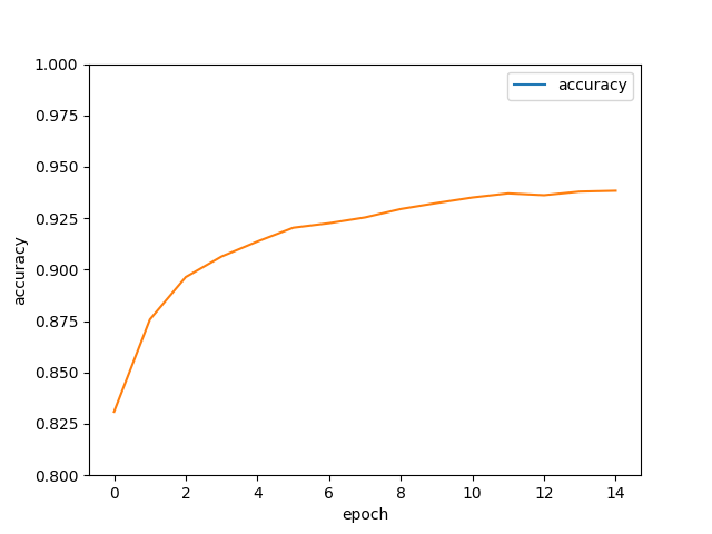
Train Epoch: 01 Loss= 6.828331470  Accuracy= 0.8309
Train Epoch: 02 Loss= 4.488496780  Accuracy= 0.8758
Train Epoch: 03 Loss= 3.577744246  Accuracy= 0.8964
Train Epoch: 04 Loss= 3.057111502  Accuracy= 0.9064
Train Epoch: 05 Loss= 2.736637831  Accuracy= 0.9137
Train Epoch: 06 Loss= 2.479548931  Accuracy= 0.9204
Train Epoch: 07 Loss= 2.278975010  Accuracy= 0.9226
Train Epoch: 08 Loss= 2.162630558  Accuracy= 0.9254
Train Epoch: 09 Loss= 2.005532503  Accuracy= 0.9295
Train Epoch: 10 Loss= 1.911731601  Accuracy= 0.9324
Train Epoch: 11 Loss= 1.785833955  Accuracy= 0.9351
Train Epoch: 12 Loss= 1.694522023  Accuracy= 0.9371
Train Epoch: 13 Loss= 1.660093784  Accuracy= 0.9362
Train Epoch: 14 Loss= 1.623517632  Accuracy= 0.938
Train Epoch: 15 Loss= 1.616030455  Accuracy= 0.9384
Train Finished takes: 36.676905393600464
Accuracy: 0.9361

## 預測錯誤的圖片
i=8   label= 5 predict= 6
i=33   label= 4 predict= 0
i=41   label= 7 predict= 3
i=59   label= 5 predict= 8
i=63   label= 3 predict= 2
i=78   label= 9 predict= 7
i=115   label= 4 predict= 6
i=121   label= 4 predict= 8
i=126   label= 0 predict= 2
i=175   label= 7 predict= 2
i=215   label= 0 predict= 2
i=241   label= 9 predict= 8
i=247   label= 4 predict= 2
i=282   label= 7 predict= 8
i=290   label= 8 predict= 4
i=320   label= 9 predict= 8
i=321   label= 2 predict= 8
i=324   label= 0 predict= 8
i=325   label= 4 predict= 9
i=333   label= 5 predict= 3
i=359   label= 9 predict= 4
i=389   label= 9 predict= 4


將隱藏層的神經元由 256 改為 1000

# 隱藏層, 1000 個神經元
h1=layer(output_dim=1000,input_dim=784, inputs=x ,activation=tf.nn.relu)

# 輸出層, 10 個神經元
y_predict=layer(output_dim=10,input_dim=1000, inputs=h1,activation=None)

剛剛的正確率為

Accuracy: 0.9361

改為 1000 後的正確率提升為

Accuracy: 0.95

建立兩個隱藏層

x = tf.compat.v1.placeholder("float", [None, 784])

# 隱藏層 h1, 1000 個神經元
h1=layer(output_dim=1000,input_dim=784, inputs=x ,activation=tf.nn.relu)

# 隱藏層 h2, 1000 個神經元
h2=layer(output_dim=1000,input_dim=1000, inputs=h1 ,activation=tf.nn.relu)

# 輸出層, 10 個神經元
y_predict=layer(output_dim=10,input_dim=1000, inputs=h2,activation=None)

正確率可提升到

Accuracy: 0.9636

References

TensorFlow 2 教學:Keras–MNIST–數字辨識

tensorflow中將label索引轉換成one-hot形式

2020/10/26

TensorFlow手寫數字辨識_CNN

TensorFlow手寫數字辨識_CNN

以 MLP 方式建立的模型,正確率約為 96%,要再進一步提升正確率,就要使用 Yann Lecun 提出的 CNN Convolutional Neural Network。

CNN 簡介

卷積運算就是將一個影像,經過卷積運算後,產生多個影像,分為兩個部分

  1. 卷積與縮減取樣,提取影像的特徵

    經過第一次卷積、第一次縮減取樣、第二次卷積、第二次縮減取樣,提取影像的特徵

  2. 完全連結神經網路

    提取影像特徵後,reshape 為1維的向量,送進 平坦層、隱藏層、輸出層 組成的累身經網路進行處理

池化層用來 downsampling,優點:

  1. 減少所需處理的資料點:減少後續運算所需時間
  2. 讓影像位置差異變小:手寫數字的位置不同,會影響辨識結果,減少影像大小可讓位置差異變小
  3. 參數的數量與計算量下降:控制 overfitting 的問題

tensorflow CNN

import tensorflow as tf
import numpy as np

# STEP 1 讀取資料
mnist = tf.keras.datasets.mnist
# Tuple of Numpy arrays: (x_train, y_train), (x_test, y_test)

(x_train, y_train), (x_test, y_test) = mnist.load_data()

# 將 training 的 input 資料 28*28 的 2維陣列 轉為 1維陣列,再轉成 float32
# 每一個圖片,都變成 784 個 float 的 array
# training 與 testing 資料數量分別是 60000 與 10000 筆
# X_train_2D 是 [60000, 28*28] 的 2維陣列
x_train_2D = x_train.reshape(60000, 28*28).astype('float32')
x_test_2D = x_test.reshape(10000, 28*28).astype('float32')
print('x_train_2D.shape=', x_train_2D.shape)
# x_train_2D.shape=(60000, 784)

# 將圖片的數字 (0~255) 標準化,最簡單的方法就是直接除以 255
# x_train_norm 是標準化後的結果,每一個數字介於 0~1 之間
x_train_norm = x_train_2D/255
x_test_norm = x_test_2D/255

# 將 training 的 label 進行 one-hot encoding,例如數字 7 經過 One-hot encoding 轉換後是 array([0., 0., 0., 0., 0., 0., 0., 1., 0., 0.], dtype=float32),即第7個值為 1

y_train_one_hot_tf=tf.one_hot(y_train,10)
y_test_one_hot_tf=tf.one_hot(y_test,10)

y_train_one_hot = None
y_test_one_hot = None
with tf.compat.v1.Session() as sess:
    init = tf.compat.v1.global_variables_initializer()
    sess.run(init)
    y_train_one_hot = sess.run(y_train_one_hot_tf)
    y_test_one_hot = sess.run(y_test_one_hot_tf)

# 將 x_train, y_train 分成 train 與 validation 兩個部分
x_train_norm_data = x_train_norm[0:50000]
x_train_norm_validation = x_train_norm[50000:60000]

y_train_one_hot_data = y_train_one_hot[0:50000]
y_train_one_hot_validation = y_train_one_hot[50000:60000]


### 建立模型

# 先建立一些共用的函數
def weight(shape):
    return tf.Variable(tf.random.truncated_normal(shape, stddev=0.1),
                       name ='W')
# bias 張量,先以 constant 建立常數,然後用 Variable 建立張量變數
def bias(shape):
    return tf.Variable(tf.constant(0.1, shape=shape)
                       , name = 'b')
# 卷積運算 功能相當於濾鏡
#  x 是輸入的影像,必須是 4 維的張量
#  W 是 filter weight 濾鏡的權重,後續以隨機方式產生 filter weight
#  strides 是 濾鏡的跨步 step,設定為 [1,1,1,1],格式是 [1, stride, stride, 1],濾鏡每次移動時,從左到右,上到下,各移動 1 步
#  padding 是 'SAME',此模式會在邊界以外 補0 再做運算,讓輸入與輸出影像為相同大小
def conv2d(x, W):
    return tf.nn.conv2d(x, W, strides=[1,1,1,1],
                        padding='SAME')

# 建立池化層,進行影像的縮減取樣
#  x 是輸入的影像,必須是 4 維的張量
#  ksize 是縮減取樣窗口的大小,設定為 [1,2,2,1],格式為 [1, height, width, 1],也就是高度 2 寬度 2 的窗口
#  stides 是縮減取樣窗口的跨步 step,設定為 [1,2,2,1],格式為 [1, stride, stride, 1],也就是縮減取樣窗口,由左到右,由上到下,各2步
#  原本 28x28 的影像,經過 max-pool 後,會縮小為 14x14
def max_pool_2x2(x):
    return tf.nn.max_pool2d(x, ksize=[1,2,2,1],
                          strides=[1,2,2,1],
                          padding='SAME')


# 輸入層
with tf.name_scope('Input_Layer'):
    # placeholder 會傳入影像
    x = tf.compat.v1.placeholder("float",shape=[None, 784],name="x")
    # x 原本為 1 維張量,要 reshape 為 4 維張量
    # 第 1 維 -1,因為後續訓練要透過 placeholder 輸入的資料筆數不固定
    # 第 2, 3 維,是 28, 28,因為影像為 28x28
    # 第 4 維是 1,因為是單色的影像,就設定為 1,如果是彩色,要設定為 3 (RGB)
    x_image = tf.reshape(x, [-1, 28, 28, 1])

# CNN Layer 1
# 用來提取特徵,卷積運算後,會產生 16 個影像,大小仍為 28x28
with tf.name_scope('C1_Conv'):
    # filter weight 大小為 5x5
    # 因為是單色,第 3 維設定為 1
    # 要產生 16 個影像,所以第 4 維設定為 16
    W1 = weight([5,5,1,16])

    # 因為產生 16 個影像,所以輸入餐次 shape = 16
    b1 = bias([16])

    # 卷積運算
    Conv1=conv2d(x_image, W1)+ b1
    # ReLU 激活函數
    C1_Conv = tf.nn.relu(Conv1 )

# 池化層用來 downsampling,將影像由 28x28 縮小為 14x14,影像數量仍為 16
with tf.name_scope('C1_Pool'):
    C1_Pool = max_pool_2x2(C1_Conv)

# CNN Layer 2
# 第二次卷積運算,將 16 個影像轉換為 36 個影像,卷積運算不改變影像大小,仍為 14x14
with tf.name_scope('C2_Conv'):
    # filter weight 大小為 5x5
    # 第 3 維是 16,因為卷積層1 的影像數量為 16
    # 第 4 維設定為 36,因為將 16 個影像轉換為 36個
    W2 = weight([5,5,16,36])
    # 因為產生 36 個影像,所以輸入餐次 shape = 36
    b2 = bias([36])
    Conv2=conv2d(C1_Pool, W2)+ b2
    # relu 會將負數的點轉換為 0
    C2_Conv = tf.nn.relu(Conv2)

# 池化層2用來 downsampling,將影像由 14x14 縮小為 7x7,影像數量仍為 36
with tf.name_scope('C2_Pool'):
    C2_Pool = max_pool_2x2(C2_Conv)

# Fully Connected Layer
# 平坦層,將 36個 7x7 影像,轉換為 1 維向量,長度為 36x7x7= 1764,也就是 1764 個 float,作為輸入資料
with tf.name_scope('D_Flat'):
    D_Flat = tf.reshape(C2_Pool, [-1, 1764])

with tf.name_scope('D_Hidden_Layer'):
    W3= weight([1764, 128])
    b3= bias([128])
    D_Hidden = tf.nn.relu(
                  tf.matmul(D_Flat, W3)+b3)

    ## Please use `rate` instead of `keep_prob`. Rate should be set to `rate = 1 - keep_prob`.
    # D_Hidden_Dropout= tf.nn.dropout(D_Hidden, keep_prob=0.8)
    D_Hidden_Dropout= tf.nn.dropout(D_Hidden, rate = 0.2)

# 輸出層, 10 個神經元
#  y_predict = softmax(D_Hidden_Dropout * W4 + b4)
with tf.name_scope('Output_Layer'):
    # 因為上一層 D_Hidden 是 128 個神經元,所以第1維是 128
    W4 = weight([128,10])
    b4 = bias([10])
    y_predict= tf.nn.softmax(
                 tf.matmul(D_Hidden_Dropout, W4)+b4)


### 設定訓練模型最佳化步驟
# 使用反向傳播演算法,訓練多層感知模型
with tf.name_scope("optimizer"):

    y_label = tf.compat.v1.placeholder("float", shape=[None, 10],
                              name="y_label")

    loss_function = tf.reduce_mean(
                      tf.nn.softmax_cross_entropy_with_logits
                         (logits=y_predict ,
                          labels=y_label))

    optimizer = tf.compat.v1.train.AdamOptimizer(learning_rate=0.0001) \
                    .minimize(loss_function)


### 設定評估模型
with tf.name_scope("evaluate_model"):
    correct_prediction = tf.equal(tf.argmax(y_predict, 1),
                                  tf.argmax(y_label, 1))
    accuracy = tf.reduce_mean(tf.cast(correct_prediction, "float"))


### 訓練模型

trainEpochs = 30
batchSize = 100
totalBatchs = int(len(x_train_norm_data)/batchSize)
epoch_list=[];accuracy_list=[];loss_list=[];
from time import time

with tf.compat.v1.Session() as sess:
    startTime=time()

    sess.run(tf.compat.v1.global_variables_initializer())

    for epoch in range(trainEpochs):
        for i in range(totalBatchs):
            # batch_x, batch_y = mnist.train.next_batch(batchSize)
            batch_x = x_train_norm_data[i*batchSize:(i+1)*batchSize]
            batch_y = y_train_one_hot_data[i*batchSize:(i+1)*batchSize]

            sess.run(optimizer,feed_dict={x: batch_x,
                                          y_label: batch_y})

        loss,acc = sess.run([loss_function,accuracy],
                            feed_dict={x: x_train_norm_validation,
                                       y_label: y_train_one_hot_validation})

        epoch_list.append(epoch)
        loss_list.append(loss)
        accuracy_list.append(acc)

        print("Train Epoch:", '%02d' % (epoch+1), "Loss=","{:.9f}".format(loss)," Accuracy=",acc)

    duration =time()-startTime
    print("Train Finished takes:",duration)

    ## 評估模型準確率
    print("Accuracy:",
      sess.run(accuracy,feed_dict={x: x_test_norm,
                                   y_label:y_test_one_hot}))
    # 前 5000 筆
    print("Accuracy:",
      sess.run(accuracy,feed_dict={x: x_test_norm[:5000],
                                   y_label: y_test_one_hot[:5000]}))
    # 後 5000 筆
    print("Accuracy:",
      sess.run(accuracy,feed_dict={x: x_test_norm[5000:],
                                   y_label: y_test_one_hot[5000:]}))

    ## 預測機率
    y_predict=sess.run(y_predict,
                   feed_dict={x: x_test_norm[:5000]})

    ## 預測結果
    prediction_result=sess.run(tf.argmax(y_predict,1),
                           feed_dict={x: x_test_norm ,
                                      y_label: y_test_one_hot})

    ## 儲存模型
    saver = tf.train.Saver()
    save_path = saver.save(sess, "saveModel/CNN_model1")
    print("Model saved in file: %s" % save_path)
    merged = tf.summary.merge_all()
    # 可將 計算圖,透過 TensorBoard 視覺化
    train_writer = tf.summary.FileWriter('log/CNN',sess.graph)


# matplotlib 列印 loss, accuracy 折線圖
import matplotlib.pyplot as plt

fig = plt.gcf()
# fig.set_size_inches(4,2)
plt.plot(epoch_list, loss_list, label = 'loss')
plt.ylabel('loss')
plt.xlabel('epoch')
plt.legend(['loss'], loc='upper left')
plt.savefig('loss.png')


fig = plt.gcf()
# fig.set_size_inches(4,2)
plt.plot(epoch_list, accuracy_list,label="accuracy" )

plt.ylim(0.8,1)
plt.ylabel('accuracy')
plt.xlabel('epoch')
plt.legend(['accuracy'], loc='upper right')
plt.savefig('accuracy.png')

############
# 查看多筆資料,以及 label
import matplotlib.pyplot as plt
def plot_images_labels_prediction(images,labels,prediction,idx,filename, num=10):
    fig = plt.gcf()
    fig.set_size_inches(12, 14)
    if num>25: num=25
    for i in range(0, num):
        ax=plt.subplot(5,5, 1+i)

        # 將 images 的 784 個數字轉換為 28x28
        ax.imshow(np.reshape(images[idx],(28, 28)), cmap='binary')

        # 轉換 one_hot label 為數字
        title= "label=" +str(np.argmax(labels[idx]))
        if len(prediction)>0:
            title+=",predict="+str(prediction[idx])

        ax.set_title(title,fontsize=10)
        ax.set_xticks([]);ax.set_yticks([])
        idx+=1
    plt.savefig(filename)


plot_images_labels_prediction(x_test_norm,
                              y_test_one_hot,
                              prediction_result,0, "result.png", num=10)

# 找出預測錯誤
for i in range(400):
    if prediction_result[i]!=np.argmax(y_test_one_hot[i]):
        print("i="+str(i)+
              "   label=",np.argmax(y_test_one_hot[i]),
              "predict=",prediction_result[i])
Train Epoch: 01 Loss= 1.604377151  Accuracy= 0.8872
Train Epoch: 02 Loss= 1.547111511  Accuracy= 0.9281
Train Epoch: 03 Loss= 1.525221825  Accuracy= 0.9447
Train Epoch: 04 Loss= 1.516423583  Accuracy= 0.9511
Train Epoch: 05 Loss= 1.507740974  Accuracy= 0.9584
Train Epoch: 06 Loss= 1.503444791  Accuracy= 0.9636
Train Epoch: 07 Loss= 1.496760130  Accuracy= 0.9683
Train Epoch: 08 Loss= 1.494633555  Accuracy= 0.9712
Train Epoch: 09 Loss= 1.492025375  Accuracy= 0.9724
Train Epoch: 10 Loss= 1.491448402  Accuracy= 0.9735
Train Epoch: 11 Loss= 1.488568783  Accuracy= 0.9751
Train Epoch: 12 Loss= 1.488826513  Accuracy= 0.9745
Train Epoch: 13 Loss= 1.485750437  Accuracy= 0.9778
Train Epoch: 14 Loss= 1.484605789  Accuracy= 0.9798
Train Epoch: 15 Loss= 1.483879209  Accuracy= 0.9788
Train Epoch: 16 Loss= 1.482506037  Accuracy= 0.9808
Train Epoch: 17 Loss= 1.482969046  Accuracy= 0.9796
Train Epoch: 18 Loss= 1.481315017  Accuracy= 0.9811
Train Epoch: 19 Loss= 1.480247617  Accuracy= 0.983
Train Epoch: 20 Loss= 1.480669379  Accuracy= 0.9817
Train Epoch: 21 Loss= 1.480412602  Accuracy= 0.9824
Train Epoch: 22 Loss= 1.479805708  Accuracy= 0.983
Train Epoch: 23 Loss= 1.479858279  Accuracy= 0.9827
Train Epoch: 24 Loss= 1.479218960  Accuracy= 0.9834
Train Epoch: 25 Loss= 1.479144573  Accuracy= 0.9829
Train Epoch: 26 Loss= 1.478820801  Accuracy= 0.9838
Train Epoch: 27 Loss= 1.477338433  Accuracy= 0.9857
Train Epoch: 28 Loss= 1.478171706  Accuracy= 0.9847
Train Epoch: 29 Loss= 1.477008104  Accuracy= 0.9856
Train Epoch: 30 Loss= 1.477438688  Accuracy= 0.9845
Train Finished takes: 1763.7836382389069
Accuracy: 0.988
Accuracy: 0.9814
Accuracy: 0.9928

i=18   label= 3 predict= 5
i=290   label= 8 predict= 4
i=321   label= 2 predict= 7
i=359   label= 9 predict= 8

2020/10/19

Keras 手寫阿拉伯數字辨識 CNN

Keras 手寫阿拉伯數字辨識 CNN

卷積神經網路 CNN 是由 Yann LeCun 提出,以下是以 CNN 進行 mnist 資料辨識。

MLP 與 CNN 的差異是 CNN 增加了卷積層1、池化層1、卷積層2、池化層2 的處理,用以提取特徵。

CNN 可分為兩個部分

  1. 影像的特徵擷取

    透過卷積層1、池化層1、卷積層2、池化層2 的處理,用以提取特徵

  2. 完全連結神經網路

    包含平坦層、隱藏層、輸出層組成的類神經網路

卷積運算的效果很類似濾鏡,擷取了不同的特徵。


卷積運算

  1. 以隨機方式產生, filter weight 大小為 3x3
  2. 將要轉換的影像,由左至右、上至下,依序選取 3x3 的矩陣
  3. 影像選取的矩陣 3x3,及 filter weight 3x3 乘積的結果,算出第一列第一行的數字
  1. 依照同樣的方式,完成所有運算

  2. 使用單一 filter weight 卷積運算產生影像

    以下是數字 7 (28x28) 的影像,使用隨機產生的 5x5 filter weight (w) 濾鏡,進行卷積運算後的結果。卷積運算不會改變圖片的大小,但運算後的結果,可提取輸入的不同特徵,ex: 邊緣、線條、角

  3. 使用多個 filter weight 卷積運算產生多個影像

    接下來隨機產生 16 個 filter weight,也就是 16 個濾鏡

    透過卷積運算,使用 16 個 filter weight,產生 16個影像,每一種影像提取了不同的特徵

  4. Max-Pool 運算

    可將影像縮減取樣 (downsampling),例如原本是 4x4 的影像,Max-Pool 後得到的影像為 2x2

  5. 使用 Max-Pool 轉換手寫數字影像

    將 16 個 28x28 影像,縮小為 16 個 14x14 的影像,影像數量不變

    Max-Pool downsampling 會縮小圖片,其優點是

    • 減少需要處理的資料點:減少運算時間
    • 讓影像位置差異變小:例如 7,在圖片中的位置不固定,可能偏某一側,但位置不同會影響辨識,減少影像大小,讓數字的位置差異變小
    • 參數的數量與計算量下降:降低發生 overfitting 的狀況

MNIST CNN

步驟

  1. 資料預處理 Preprocess:處理後產生 features (影像特徵值)與 label (數字的真實值)

  2. 建立模型:建立 CNN model

  3. 訓練模型:輸入 features, label,執行 10 次訓練週期

  4. 評估模型準確率:使用測試資料評估模型準確率

  5. 預測:利用 model,輸入測試資料進行預測

from keras.datasets import mnist
from keras.utils import np_utils
import numpy as np
np.random.seed(10)

## step 1 資料預處理 Preprocess:處理後產生 features (影像特徵值)與 label (數字的真實值)
# 讀取 mnist 資料
(x_Train, y_Train), (x_Test, y_Test) = mnist.load_data()
# 將 features (影像特徵值),轉換為 4 維矩陣
# 將 features,以 reshape 轉為 6000 x 28 x 28 x 1 的 4 維矩陣
x_Train4D = x_Train.reshape(x_Train.shape[0],28,28,1).astype('float32')
x_Test4D = x_Test.reshape(x_Test.shape[0],28,28,1).astype('float32')

# 將 features 標準化
x_Train4D_normalize = x_Train4D / 255
x_Test4D_normalize = x_Test4D / 255

# 以 Onehot Encoding 轉換 label
y_TrainOneHot = np_utils.to_categorical(y_Train)
y_TestOneHot = np_utils.to_categorical(y_Test)

#########
## step 2 建立模型:建立 CNN model
from keras.models import Sequential
from keras.layers import Dense,Dropout,Flatten,Conv2D,MaxPooling2D

# 線性堆疊模型
model = Sequential()

# 建立卷積層1
# 輸入數字影像 28x28 的大小,執行一次卷積運算,產生 16 個影像,卷積運算不會改變影像大小,結果還是 28x28
# filters=16             建立 16 個 filter weight
# kernel_size=(5,5)      每一個濾鏡大小為 5x5
# padding='same'         讓卷積運算產生的影像大小不變
# input_shape=(28,28,1)  第1, 2 維,是輸入的影像形狀 28x28,第 3 維,因為是單色灰階影像,所以是 1
# activation='relu'      設定 ReLU 激活函數
model.add(Conv2D(filters=16,
                 kernel_size=(5,5),
                 padding='same',
                 input_shape=(28,28,1),
                 activation='relu'))

# 建立池化層
# 輸入參數 pool_size=(2, 2),執行第一次縮減取樣,將 16 個 28x28 影像,縮小為 16 個 14x14 的影像
model.add(MaxPooling2D(pool_size=(2, 2)))

# 建立卷積層2
# 執行第二次卷積運算,將原本的 16 個影像,轉換為 36 個影像,卷積運算不會改變影像大小,結果還是 14x14
model.add(Conv2D(filters=36,
                 kernel_size=(5,5),
                 padding='same',
                 activation='relu'))

# 建立池化層2,並加入Dropout 避免 overfitting
# 執行第二次縮減取樣,將 36 個 14x14 的影像,縮小為 36 個 7x7 的影像
model.add(MaxPooling2D(pool_size=(2, 2)))
model.add(Dropout(0.25))

# 建立神經網路 (平坦層, 隱藏層, 輸出層)
# 建立平坦層
# 根據池化層2 的結果,共36 個 7x7 影像,轉換為 1維向量,長度是 36x7x7=1764,也就是 1764 個 float,正好對應到 1764 個神經元
model.add(Flatten())
# 建立隱藏層,共有 128 個神經元
model.add(Dense(128, activation='relu'))
# 加入 Dropout(0.5)
# 每次訓練迭代時,會隨機在神經網路中,放棄 50% 的神經元,以避免 overfitting
model.add(Dropout(0.5))
# 建立輸出層
# 共 10 個神經元,對應 0~9 共 10 個數字,並使用 softmax 激活函數進行轉換
# softmax 可將神經元的輸出,轉換為預測每一個數字的機率
model.add(Dense(10,activation='softmax'))

print(model.summary())

#######
## 訓練模型:輸入 features, label,執行 10 次訓練週期
model.compile(loss='categorical_crossentropy',
              optimizer='adam',metrics=['accuracy'])

# validation_split=0.2   80% 為訓練資料, 20% 驗證資料
# batch_size=300         每一批次300 筆資料
# verbose=2              顯示訓練過程
train_history=model.fit(x=x_Train4D_normalize,
                        y=y_TrainOneHot,validation_split=0.2,
                        epochs=20, batch_size=300,verbose=2)


# 模型訓練結果 結構存檔
from keras.models import model_from_json
json_string = model.to_json()
with open("model.config", "w") as text_file:
    text_file.write(json_string)

# 模型訓練結果 權重存檔
model.save_weights("model.weight")


import matplotlib.pyplot as plt
def save_train_history(train_acc,test_acc, filename):
    plt.clf()
    plt.plot(train_history.history[train_acc])
    plt.plot(train_history.history[test_acc])
    plt.title('Train History')
    plt.ylabel('Accuracy')
    plt.xlabel('Epoch')
    plt.legend(['train', 'test'], loc='upper left')
    plt.savefig(filename)


save_train_history('accuracy','val_accuracy', 'acc.png')

save_train_history('loss','val_loss', 'loss.png')


#####
# step 4 評估模型準確率:使用測試資料評估模型準確率

scores = model.evaluate(x_Test4D_normalize , y_TestOneHot)
scores[1]

#####
# step 5 預測:利用 model,輸入測試資料進行預測
prediction=model.predict_classes(x_Test4D_normalize)
prediction[:10]

# 查看預測結果
import matplotlib.pyplot as plt
def plot_images_labels_prediction(images,labels,prediction,filename, idx, num=10):
    fig = plt.gcf()
    fig.set_size_inches(12, 14)
    if num>25: num=25
    for i in range(0, num):
        ax=plt.subplot(5,5, 1+i)
        ax.imshow(images[idx], cmap='binary')

        ax.set_title("label=" +str(labels[idx])+
                     ",predict="+str(prediction[idx])
                     ,fontsize=10)

        ax.set_xticks([]);ax.set_yticks([])
        idx+=1
    plt.savefig(filename)

plot_images_labels_prediction(x_Test,y_Test,prediction, 'predict.png', idx=0)

####
# confusion maxtrix

import pandas as pd
crosstab1 = pd.crosstab(y_Test,prediction,
            rownames=['label'],colnames=['predict'])

print()
print(crosstab1)

df = pd.DataFrame({'label':y_Test, 'predict':prediction})

df[(df.label==5)&(df.predict==3)]

列印 model

Model: "sequential_1"
_________________________________________________________________
Layer (type)                 Output Shape              Param #
=================================================================
conv2d_1 (Conv2D)            (None, 28, 28, 16)        416
_________________________________________________________________
max_pooling2d_1 (MaxPooling2 (None, 14, 14, 16)        0
_________________________________________________________________
conv2d_2 (Conv2D)            (None, 14, 14, 36)        14436
_________________________________________________________________
max_pooling2d_2 (MaxPooling2 (None, 7, 7, 36)          0
_________________________________________________________________
dropout_1 (Dropout)          (None, 7, 7, 36)          0
_________________________________________________________________
flatten_1 (Flatten)          (None, 1764)              0
_________________________________________________________________
dense_1 (Dense)              (None, 128)               225920
_________________________________________________________________
dropout_2 (Dropout)          (None, 128)               0
_________________________________________________________________
dense_2 (Dense)              (None, 10)                1290
=================================================================
Total params: 242,062
Trainable params: 242,062
Non-trainable params: 0

訓練過程,可發現 loss 越來越小,accuracy 越來越高

Train on 48000 samples, validate on 12000 samples
Epoch 1/20
 - 58s - loss: 0.4736 - accuracy: 0.8517 - val_loss: 0.1006 - val_accuracy: 0.9694
Epoch 2/20
 - 63s - loss: 0.1326 - accuracy: 0.9604 - val_loss: 0.0652 - val_accuracy: 0.9813
Epoch 3/20
 - 65s - loss: 0.0980 - accuracy: 0.9700 - val_loss: 0.0555 - val_accuracy: 0.9838
Epoch 4/20
 - 67s - loss: 0.0791 - accuracy: 0.9761 - val_loss: 0.0479 - val_accuracy: 0.9862
Epoch 5/20
 - 61s - loss: 0.0698 - accuracy: 0.9779 - val_loss: 0.0442 - val_accuracy: 0.9873
Epoch 6/20
 - 59s - loss: 0.0616 - accuracy: 0.9813 - val_loss: 0.0434 - val_accuracy: 0.9875
Epoch 7/20
 - 62s - loss: 0.0531 - accuracy: 0.9835 - val_loss: 0.0370 - val_accuracy: 0.9893
Epoch 8/20
 - 63s - loss: 0.0496 - accuracy: 0.9843 - val_loss: 0.0363 - val_accuracy: 0.9904
Epoch 9/20
 - 61s - loss: 0.0455 - accuracy: 0.9863 - val_loss: 0.0347 - val_accuracy: 0.9908
Epoch 10/20
 - 65s - loss: 0.0417 - accuracy: 0.9870 - val_loss: 0.0319 - val_accuracy: 0.9920
Epoch 11/20
 - 69s - loss: 0.0375 - accuracy: 0.9880 - val_loss: 0.0309 - val_accuracy: 0.9912
Epoch 12/20
 - 62s - loss: 0.0357 - accuracy: 0.9891 - val_loss: 0.0341 - val_accuracy: 0.9907
Epoch 13/20
 - 73s - loss: 0.0347 - accuracy: 0.9894 - val_loss: 0.0332 - val_accuracy: 0.9909
Epoch 14/20
 - 64s - loss: 0.0314 - accuracy: 0.9902 - val_loss: 0.0312 - val_accuracy: 0.9921
Epoch 15/20
 - 65s - loss: 0.0298 - accuracy: 0.9907 - val_loss: 0.0296 - val_accuracy: 0.9923
Epoch 16/20
 - 66s - loss: 0.0260 - accuracy: 0.9914 - val_loss: 0.0312 - val_accuracy: 0.9920
Epoch 17/20
 - 69s - loss: 0.0255 - accuracy: 0.9923 - val_loss: 0.0270 - val_accuracy: 0.9933
Epoch 18/20
 - 67s - loss: 0.0243 - accuracy: 0.9924 - val_loss: 0.0305 - val_accuracy: 0.9921
Epoch 19/20
 - 62s - loss: 0.0241 - accuracy: 0.9922 - val_loss: 0.0299 - val_accuracy: 0.9925
Epoch 20/20
 - 71s - loss: 0.0214 - accuracy: 0.9933 - val_loss: 0.0311 - val_accuracy: 0.9918

訓練與驗證的準確率都越來越高,誤差越來越低,且沒有 overfitting 的現象

預測的 scores,準確率 0.9926

[0.021972040887850517, 0.9926000237464905]

這是前 10 筆預測資料

crosstab 結果

predict    0     1     2    3    4    5    6     7    8    9
label
0        976     1     0    0    0    0    1     1    1    0
1          0  1133     1    0    0    0    0     1    0    0
2          2     0  1024    0    0    0    0     4    2    0
3          0     0     1  999    0    3    0     2    3    2
4          0     0     0    0  978    0    1     0    0    3
5          1     0     0    4    0  883    3     0    0    1
6          3     2     0    0    2    1  949     0    1    0
7          0     2     3    0    0    0    0  1022    1    0
8          3     1     1    1    0    0    0     0  967    1
9          1     0     0    0    6    2    0     4    1  995

References

TensorFlow+Keras深度學習人工智慧實務應用

何時使用MLP,CNN和RNN神經網絡