迴歸
學習資料
取得學習資料文字檔 click.csv
x,y
235,591
216,539
148,413
35,310
85,308
...
先利用 matplotlib 繪製到圖表上
import numpy as np
import matplotlib.pyplot as plt

train = np.loadtxt('click.csv', delimiter=',', skiprows=1)
train_x = train[:,0]
train_y = train[:,1]

plt.plot(train_x, train_y, 'o')
plt.show()
另外針對原始的學習資料,進行標準化(z-score正規化),也就是將資料平均轉換為 0,分散轉換為1。其中 𝜇 是所有資料的平均,𝜎 是所有資料的標準差。這樣處理後,會讓參數收斂更快。
\(z^{(i)} = \frac{x^{(i)} - 𝜇}{𝜎}\)
import numpy as np
import matplotlib.pyplot as plt

train = np.loadtxt('click.csv', delimiter=',', skiprows=1)
train_x = train[:,0]
train_y = train[:,1]

# 標準化
mu = train_x.mean()
sigma = train_x.std()
def standardize(x):
    return (x - mu) / sigma

train_z = standardize(train_x)

plt.plot(train_z, train_y, 'o')
plt.show()

一次函數
先使用一次目標函數 \(f_𝜃(x)\)
\({f_𝜃(x)=𝜃_0+𝜃_1x}\)
\({E(𝜃)= \frac{1}{2} \sum_{i=1}^{n}( y^{(i)} - f_𝜃(x^{(i)})^2 }\)
\(𝜃_0, 𝜃_1\) 可任意選擇初始值
\(𝜃_0, 𝜃_1\) 的參數更新式為
\(𝜃_0 := 𝜃_0 - 𝜂 \sum_{i=1}^{n}( f_𝜃(x^{(i)} )-y^{(i)} )\)
\(𝜃_1 := 𝜃_1 - 𝜂 \sum_{i=1}^{n}( f_𝜃(x^{(i)} )-y^{(i)} )x^{(i)}\)
用這個方法,就可以找出正確的 \(𝜃_0, 𝜃_1\)
其中 𝜂 是任意數值,先設定為 \(10^{-3}\) 試試看。一般來說,會指定要處理的次數,有時會比較參數更新前後,目標函數的值,如果差異不大,就直接結束。另外 \(𝜃_0, 𝜃_1\) 必須同時一起更新。
import numpy as np
import matplotlib.pyplot as plt

# 載入學習資料
train = np.loadtxt('click.csv', delimiter=',', dtype='int', skiprows=1)
train_x = train[:,0]
train_y = train[:,1]

# 標準化
mu = train_x.mean()
sigma = train_x.std()
def standardize(x):
    return (x - mu) / sigma

train_z = standardize(train_x)

# 任意選擇初始值
theta0 = np.random.rand()
theta1 = np.random.rand()

# 預測函數
def f(x):
    return theta0 + theta1 * x

# 目標函數 E(𝜃)
def E(x, y):
    return 0.5 * np.sum((y - f(x)) ** 2)

# 學習率
ETA = 1e-3

# 誤差
diff = 1

# 更新次數
count = 0

# 重複學習
error = E(train_z, train_y)
while diff > 1e-2:
    # 暫存更新結果
    tmp_theta0 = theta0 - ETA * np.sum((f(train_z) - train_y))
    tmp_theta1 = theta1 - ETA * np.sum((f(train_z) - train_y) * train_z)

    # 更新參數
    theta0 = tmp_theta0
    theta1 = tmp_theta1

    # 計算誤差
    current_error = E(train_z, train_y)
    diff = error - current_error
    error = current_error

    # log
    count += 1
    log = '{}次數: theta0 = {:.3f}, theta1 = {:.3f}, 誤差 = {:.4f}'
    print(log.format(count, theta0, theta1, diff))

# 繪製學習資料與預測函數的直線
x = np.linspace(-3, 3, 100)
plt.plot(train_z, train_y, 'o')
plt.plot(x, f(x))
plt.show()
測試結果
391次數: theta0 = 428.991, theta1 = 93.444, 誤差 = 0.0109
392次數: theta0 = 428.994, theta1 = 93.445, 誤差 = 0.0105
393次數: theta0 = 428.997, theta1 = 93.446, 誤差 = 0.0101
394次數: theta0 = 429.000, theta1 = 93.446, 誤差 = 0.0097
驗證
可輸入 x 預測點擊數,但因為剛剛有將學習資料正規化,預測資料也必須正規化
>>> f(standardize(100))
370.96741051658194
>>> f(standardize(500))
928.9775823086377
二次多項式迴歸
\(f_𝜃(x) = 𝜃_0 + 𝜃_1x + 𝜃_2x^2\) 要增加 \( 𝜃_2\) 這個參數
目標的誤差函數 \({E(𝜃)= \frac{1}{2} \sum_{i=1}^{n}( y^{(i)} - f_𝜃(x^{(i)})^2 }\)
因為有多筆學習資料,可將資料以矩陣方式處理
\( X = \begin{bmatrix}
(x^{(1)})^T\\
(x^{(2)})^T\\
\cdot \\
\cdot \\
(x^{(n)})^T \\
\end{bmatrix}
= \begin{bmatrix}
1 & x^{(1)} & (x^{(1)})^2 \\
1 & x^{(2)} & (x^{(2)})^2 \\
\cdot \\
\cdot \\
1 & x^{(n)} & (x^{(n)})^2 \\
\end{bmatrix} \)
\(f_𝜃(x) = \begin{bmatrix}
1 & x^{(1)} & (x^{(1)})^2 \\
1 & x^{(2)} & (x^{(2)})^2 \\
\cdot \\
\cdot \\
1 & x^{(n)} & (x^{(n)})^2 \\
\end{bmatrix} \begin{bmatrix}
𝜃_0 \\
𝜃_1 \\
𝜃_2 \\
\end{bmatrix}
= \begin{bmatrix}
𝜃_0 + 𝜃_1 x^{(1)} + 𝜃_2 (x^{(1)})^2\\
𝜃_0 + 𝜃_1 x^{(2)} + 𝜃_2 (x^{(2)})^2\\
\cdot \\
\cdot \\
𝜃_0 + 𝜃_1 x^{(n)} + 𝜃_2 (x^{(n)})^2\\
\end{bmatrix}\)
第j 項參數的更新式定義為
\(𝜃_j := 𝜃_j - 𝜂 \sum_{i=1}^{n}( f_𝜃(x^{(i)} )-y^{(i)} )x_j^{(i)}\)
可將 \( ( f_𝜃(x^{(i)} )-y^{(i)} ) \) 以及 \(x_j^{(i)}\) 這兩部分各自以矩陣方式處理
\( f= \begin{bmatrix}
( f_𝜃(x^{(1)} )-y^{(1)} )\\
( f_𝜃(x^{(2)} )-y^{(2)} )\\
\cdot \\
\cdot \\
( f_𝜃(x^{(n)} )-y^{(n)} ) \\
\end{bmatrix} \)
\( x_0 = \begin{bmatrix}
x_0^{(1)} \\
x_0^{(2)}\\
\cdot \\
\cdot \\
x_0^{(n)} \\
\end{bmatrix} \)
\( \sum_{i=1}^{n}( f_𝜃(x^{(i)} )-y^{(i)} )x_0^{(i)} = f^Tx_0 \)
分別考慮三個參數
\( x_0 = \begin{bmatrix}
x_0^{(1)} \\
x_0^{(2)}\\
\cdot \\
\cdot \\
x_0^{(n)} \\
\end{bmatrix} ,
x_1 = \begin{bmatrix}
x^{(1)} \\
x^{(2)}\\
\cdot \\
\cdot \\
x^{(n)} \\
\end{bmatrix} ,
x_2 = \begin{bmatrix}
(x^{(1)})^2 \\
(x^{(2)})^2\\
\cdot \\
\cdot \\
(x^{(n)})^2 \\
\end{bmatrix}\)
\( X = \begin{bmatrix}
x_0 & x_1 & x_2
\end{bmatrix}
= \begin{bmatrix}
1 & x^{(1)} & (x^{(1)})^2 \\
1 & x^{(2)} & (x^{(2)})^2\\
\cdot \\
\cdot \\
1 & x^{(n)} & (x^{(n)})^2 \\
\end{bmatrix} \)
使用 \( f^TX\) 就可以一次更新三個參數
import numpy as np
import matplotlib.pyplot as plt

# 讀取學習資料
train = np.loadtxt('click.csv', delimiter=',', dtype='int', skiprows=1)
train_x = train[:,0]
train_y = train[:,1]

# 標準化
mu = train_x.mean()
sigma = train_x.std()
def standardize(x):
    return (x - mu) / sigma

train_z = standardize(train_x)

# 任意初始值
theta = np.random.rand(3)

# 學習資料轉換為矩陣
def to_matrix(x):
    return np.vstack([np.ones(x.size), x, x ** 2]).T

X = to_matrix(train_z)

# 預測函數
def f(x):
    return np.dot(x, theta)

# 目標函數
def E(x, y):
    return 0.5 * np.sum((y - f(x)) ** 2)

# 學習率
ETA = 1e-3

# 誤差
diff = 1

# 更新次數
count = 0

# 重複學習
error = E(X, train_y)
while diff > 1e-2:
    # 更新參數
    theta = theta - ETA * np.dot(f(X) - train_y, X)

    # 計算誤差
    current_error = E(X, train_y)
    diff = error - current_error
    error = current_error

    # log
    count += 1
    log = '{}次: theta = {}, 誤差 = {:.4f}'
    print(log.format(count, theta, diff))

# 繪製學習資料與預測函數
x = np.linspace(-3, 3, 100)
plt.plot(train_z, train_y, 'o')
plt.plot(x, f(to_matrix(x)))
plt.show()
也可以將重複停止的條件,改為均方誤差
目標的誤差函數 \({E(𝜃)= \frac{1}{n} \sum_{i=1}^{n}( y^{(i)} - f_𝜃(x^{(i)})^2 }\)
import numpy as np
import matplotlib.pyplot as plt

# 讀取學習資料
train = np.loadtxt('click.csv', delimiter=',', dtype='int', skiprows=1)
train_x = train[:,0]
train_y = train[:,1]

# 標準化
mu = train_x.mean()
sigma = train_x.std()
def standardize(x):
    return (x - mu) / sigma

train_z = standardize(train_x)

# 任意初始值
theta = np.random.rand(3)

# 學習資料轉換為矩陣
def to_matrix(x):
    return np.vstack([np.ones(x.size), x, x ** 2]).T

X = to_matrix(train_z)

# 預測函數
def f(x):
    return np.dot(x, theta)

# 目標函數
def MSE(x, y):
    return ( 1 / x.shape[0] * np.sum( (y-f(x)))**2 )

# 學習率
ETA = 1e-3

# 誤差
diff = 1

# 更新次數
count = 0

# 均方誤差的歷史資料
errors = []

# 重複學習
errors.append( MSE(X, train_y) )
while diff > 1e-2:
    # 更新參數
    theta = theta - ETA * np.dot(f(X) - train_y, X)

    # 計算誤差
    errors.append( MSE(X, train_y) )
    diff = errors[-2] - errors[-1]

    # log
    count += 1
    log = '{}次: theta = {}, 誤差 = {:.4f}'
    print(log.format(count, theta, diff))

# 繪製重複次數 與誤差的關係
x = np.arange(len(errors))
plt.plot(x, errors)
plt.show()
隨機梯度下降法
隨機選擇一項學習資料,套用在參數的更新上,例如選擇第 k 項。
\(𝜃_j := 𝜃_j - 𝜂 ( f_𝜃(x^{(k)} )-y^{(k)} )x_j^{(k)}\)
import numpy as np
import matplotlib.pyplot as plt

# 載入學習資料
train = np.loadtxt('click.csv', delimiter=',', dtype='int', skiprows=1)
train_x = train[:,0]
train_y = train[:,1]

# 標準化
mu = train_x.mean()
sigma = train_x.std()
def standardize(x):
    return (x - mu) / sigma

train_z = standardize(train_x)

# 任意選擇初始值
theta = np.random.rand(3)

# 學習資料轉換為矩陣
def to_matrix(x):
    return np.vstack([np.ones(x.size), x, x ** 2]).T

X = to_matrix(train_z)

# 預測函數
def f(x):
    return np.dot(x, theta)

# 均方差
def MSE(x, y):
    return (1 / x.shape[0]) * np.sum((y - f(x)) ** 2)

# 學習率
ETA = 1e-3

# 誤差
diff = 1

# 更新次數
count = 0

# 重複學習
error = MSE(X, train_y)
while diff > 1e-2:
    # 排列學習資料所需的隨機排列
    p = np.random.permutation(X.shape[0])
    # 將學習資料以隨機方式取出,並用隨機梯度下降法 更新參數
    for x, y in zip(X[p,:], train_y[p]):
        theta = theta - ETA * (f(x) - y) * x

    # 計算跟前一個誤差的差距
    current_error = MSE(X, train_y)
    diff = error - current_error
    error = current_error

    # log
    count += 1
    log = '{}回目: theta = {}, 差分 = {:.4f}'
    print(log.format(count, theta, diff))

# 列印結果
x = np.linspace(-3, 3, 100)
plt.plot(train_z, train_y, 'o')
plt.plot(x, f(to_matrix(x)))
plt.show()
多元迴歸
如果要處理多元迴歸,就跟多項式迴歸一樣改用矩陣,但在多元迴歸中要注意,要對所有變數 \(x_1, x_2, x_3\)都進行標準化。
\(z_1^{(i)} = \frac{x_1^{(i)} - 𝜇_1}{𝜎_1} \)
\(z_2^{(i)} = \frac{x_2^{(i)} - 𝜇_2}{𝜎_2} \)
\(z_3^{(i)} = \frac{x_3^{(i)} - 𝜇_3}{𝜎_3} \)
分類(感知器)
使用 images1.csv 資料
x1,x2,y
153,432,-1
220,262,-1
118,214,-1
474,384,1
485,411,1
233,430,-1
...
先將原始資料標記在圖表上,y=1 用圓圈,y=-1 用
import numpy as np
import matplotlib.pyplot as plt

# 載入學習資料
train = np.loadtxt('images1.csv', delimiter=',', skiprows=1)
train_x = train[:,0:2]
train_y = train[:,2]

# 繪圖
x1 = np.arange(0, 500)
plt.plot(train_x[train_y ==  1, 0], train_x[train_y ==  1, 1], 'o')
plt.plot(train_x[train_y == -1, 0], train_x[train_y == -1, 1], 'x')
plt.savefig('1.png')
- 識別函數 \(f_w(x)\) 就是給定向量 \(x\) 後,回傳 1 或 -1 的函數,用來判斷橫向或縱向。
\(f_w(x) = \left\{\begin{matrix} 1 \quad (w \cdot x \geq 0) \\ -1 \quad (w \cdot x < 0) \end{matrix}\right.\)
- 權重更新式
\(w := \left\{\begin{matrix} w + y^{(i)}x^{(i)} \quad (f_w(x) \neq y^{(i)}) \\ w \quad \quad \quad \quad (f_w(x) = y^{(i)}) \end{matrix}\right.\)
感知器使用精度作為停止的標準比較好,但目前先直接設定訓練次數
最後繪製以權重向量為法線的直線方程式
\(w \cdot x = w_1x_1 + w_2x_2 = 0\)
\(x_2 = - \frac{w_1}{w2} x_1\)
import numpy as np
import matplotlib.pyplot as plt

# 載入學習資料
train = np.loadtxt('images1.csv', delimiter=',', skiprows=1)
train_x = train[:,0:2]
train_y = train[:,2]

# 任意初始值
w = np.random.rand(2)

# 識別函數,判斷矩形是橫向或縱向
def f(x):
    if np.dot(w, x) >= 0:
        return 1
    else:
        return -1

# 重複次數
epoch = 10

# 更新次數
count = 0

# 學習權重
for _ in range(epoch):
    for x, y in zip(train_x, train_y):
        if f(x) != y:
            w = w + y * x

            # log
            count += 1
            print('{}次數: w = {}'.format(count, w))

# 繪圖
x1 = np.arange(0, 500)
plt.plot(train_x[train_y ==  1, 0], train_x[train_y ==  1, 1], 'o')
plt.plot(train_x[train_y == -1, 0], train_x[train_y == -1, 1], 'x')
plt.plot(x1, -w[0] / w[1] * x1, linestyle='dashed')
plt.savefig("1.png")
驗證
python -i classification1_perceptron.py
>>> f([200,100])
1
>>> f([100,200])
-1
分類(邏輯迴歸)
邏輯迴歸要先修改學習資料,橫向為 1 ,縱向為 0
x1,x2,y
153,432,0
220,262,0
118,214,0
474,384,1
485,411,1
...
預測函數就是 S 函數
\(f_𝜃(x) = \frac{1}{1 + exp(-𝜃^Tx)}\)
參數更新式為
\(𝜃_j := 𝜃_j - 𝜂 \sum_{i=1}^{n}( f_𝜃(x^{(i)}) - y^{(i)} )x_j^{(i)}\)
可用矩陣處理,轉換時要加上 \(x_0\),且設定為 1,如果當 \(f_𝜃(x) \geq 0.5\),也就是 \(𝜃^T x >0\) ,就判定為橫向。
將 \(Q^Tx = 0 \) 整理後,就可得到一條直線
\(Q^Tx = 𝜃_0x_0 + 𝜃_1x_1 + 𝜃_2x_2 = 𝜃_0 +𝜃_1x_1+𝜃_2x_2 =0\)
\(x_2 = - \frac{𝜃_0 + 𝜃_1x_2}{𝜃_2}\)
import numpy as np
import matplotlib.pyplot as plt

# 載入學習資料
train = np.loadtxt('images2.csv', delimiter=',', skiprows=1)
train_x = train[:,0:2]
train_y = train[:,2]

# 任意初始值
theta = np.random.rand(3)

# 以平均及標準差進行標準化
mu = train_x.mean(axis=0)
sigma = train_x.std(axis=0)
def standardize(x):
    return (x - mu) / sigma

train_z = standardize(train_x)

# 轉換為矩陣,加上 x0
def to_matrix(x):
    x0 = np.ones([x.shape[0], 1])
    return np.hstack([x0, x])

X = to_matrix(train_z)

# 預測函數 S函數
def f(x):
    return 1 / (1 + np.exp(-np.dot(x, theta)))

# 識別函數
def classify(x):
    return (f(x) >= 0.5).astype(np.int)

# 學習率
ETA = 1e-3

# 重複次數
epoch = 5000

# 更新次數
count = 0

# 重複學習
for _ in range(epoch):
    theta = theta - ETA * np.dot(f(X) - train_y, X)

    # log
    count += 1
    print('{}次數: theta = {}'.format(count, theta))

# 繪製圖形
x0 = np.linspace(-2, 2, 100)
plt.plot(train_z[train_y == 1, 0], train_z[train_y == 1, 1], 'o')
plt.plot(train_z[train_y == 0, 0], train_z[train_y == 0, 1], 'x')
plt.plot(x0, -(theta[0] + theta[1] * x0) / theta[2], linestyle='dashed')
# plt.show()
plt.savefig("機器學習4_coding_.png")
驗證
這樣的意思是 200x100 的矩形有 91.6% 的機率會是橫向
>>> f(to_matrix(standardize([[200,100], [100,200]])))
array([0.91604483, 0.03009514])
可再轉化為 1 與 0
>>> classify(to_matrix(standardize([[200,100], [100,200]])))
array([1, 0])
線性不可分離的分類
學習資料為 data3.csv
x1,x2,y
0.54508775,2.34541183,0
0.32769134,13.43066561,0
4.42748117,14.74150395,0
2.98189041,-1.81818172,1
4.02286274,8.90695686,1
2.26722613,-6.61287392,1
-2.66447221,5.05453871,1
-1.03482441,-1.95643469,1
4.06331548,1.70892541,1
2.89053966,6.07174283,0
2.26929206,10.59789814,0
4.68096051,13.01153161,1
1.27884366,-9.83826738,1
-0.1485496,12.99605136,0
-0.65113893,10.59417745,0
3.69145079,3.25209182,1
-0.63429623,11.6135625,0
0.17589959,5.84139826,0
0.98204409,-9.41271559,1
-0.11094911,6.27900499,0
先將學習資料繪製到圖表上看起來無法用一條直線來分類,增加 \(x_1^2\) 進行分類

參數變成四個,將 \(Q^Tx = 0 \) 整理後,就可得到一條曲線
\(Q^Tx = 𝜃_0x_0 + 𝜃_1x_1 + 𝜃_2x_2 +𝜃_3x_1^2 = 𝜃_0 +𝜃_1x_1+𝜃_2x_2 +𝜃_3x_1^2 =0\)
\(x_2 = - \frac{𝜃_0 + 𝜃_1x_2 +𝜃_3x_1^2}{𝜃_2}\)
import numpy as np
import matplotlib.pyplot as plt

# 載入學習資料
train = np.loadtxt('data3.csv', delimiter=',', skiprows=1)
train_x = train[:,0:2]
train_y = train[:,2]

# 任意初始值
theta = np.random.rand(4)

# 標準化
mu = train_x.mean(axis=0)
sigma = train_x.std(axis=0)
def standardize(x):
    return (x - mu) / sigma

train_z = standardize(train_x)

# 轉換為矩陣,加上 x0, x3
def to_matrix(x):
    x0 = np.ones([x.shape[0], 1])
    x3 = x[:,0,np.newaxis] ** 2
    return np.hstack([x0, x, x3])

X = to_matrix(train_z)

# 預測函數 S函數
def f(x):
    return 1 / (1 + np.exp(-np.dot(x, theta)))

# 識別函數
def classify(x):
    return (f(x) >= 0.5).astype(np.int)

# 學習率
ETA = 1e-3

# 重複次數
epoch = 5000

# 更新次數
count = 0

# 重複學習
for _ in range(epoch):
    theta = theta - ETA * np.dot(f(X) - train_y, X)

    # log
    count += 1
    print('{}次數: theta = {}'.format(count, theta))

# 繪製圖形
x1 = np.linspace(-2, 2, 100)
x2 = -(theta[0] + theta[1] * x1 + theta[3] * x1 ** 2) / theta[2]
plt.plot(train_z[train_y == 1, 0], train_z[train_y == 1, 1], 'o')
plt.plot(train_z[train_y == 0, 0], train_z[train_y == 0, 1], 'x')
plt.plot(x1, x2, linestyle='dashed')
# plt.show()
plt.savefig("機器學習4_coding_.png")

分類的精度,就是在全部的資料中,能夠被正確分類的 TP與 TN 佔的比例,可表示為
\( Accuracy = \frac{TP + TN}{TP+FP+FN+TN} \)
# 精度
accuracies = []

# 重複學習
for _ in range(epoch):
    theta = theta - ETA * np.dot(f(X) - train_y, X)

    # 計算精度
    result = classify(X) == train_y
    accuracy = len(result[result ==True]) / len(result)
    accuracies.append(accuracy)

# 繪製圖形
x = np.arange(len(accuracies))
plt.plot(x, accuracies)
plt.savefig("機器學習4_coding_.png")
計算精度,繪製圖表

隨機梯度下降法
import numpy as np
import matplotlib.pyplot as plt

# 載入學習資料
train = np.loadtxt('data3.csv', delimiter=',', skiprows=1)
train_x = train[:,0:2]
train_y = train[:,2]

# 任意初始值
theta = np.random.rand(4)

# 標準化
mu = train_x.mean(axis=0)
sigma = train_x.std(axis=0)
def standardize(x):
    return (x - mu) / sigma

train_z = standardize(train_x)

# 轉換為矩陣,加上 x0, x3
def to_matrix(x):
    x0 = np.ones([x.shape[0], 1])
    x3 = x[:,0,np.newaxis] ** 2
    return np.hstack([x0, x, x3])

X = to_matrix(train_z)

# 預測函數 S函數
def f(x):
    return 1 / (1 + np.exp(-np.dot(x, theta)))

# 識別函數
def classify(x):
    return (f(x) >= 0.5).astype(np.int)

# 學習率
ETA = 1e-3

# 重複次數
epoch = 5000

# 更新次數
count = 0

# 重複學習
for _ in range(epoch):
    # 以隨機梯度下降法更新參數
    p = np.random.permutation(X.shape[0])
    for x, y in zip(X[p,:], train_y[p]):
        theta = theta - ETA * (f(x) - y) * x

    # log
    count += 1
    print('{}次數: theta = {}'.format(count, theta))

# 繪製圖形
x1 = np.linspace(-2, 2, 100)
x2 = -(theta[0] + theta[1] * x1 + theta[3] * x1 ** 2) / theta[2]
plt.plot(train_z[train_y == 1, 0], train_z[train_y == 1, 1], 'o')
plt.plot(train_z[train_y == 0, 0], train_z[train_y == 0, 1], 'x')
plt.plot(x1, x2, linestyle='dashed')
# plt.show()
plt.savefig("機器學習4_coding_.png")

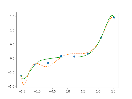
正規化
首先考慮這樣的函數
\(g(x) = 0.1(x^3 + x^2 + x)\)
產生一些雜訊的學習資料,並繪製圖表

import numpy as np
import matplotlib.pyplot as plt

# 原始真正的函數
def g(x):
    return 0.1 * (x ** 3 + x ** 2 + x)

# 適當地利用原本的函數,加上一些雜訊,產生學習資料
train_x = np.linspace(-2, 2, 8)
train_y = g(train_x) + np.random.randn(train_x.size) * 0.05


plt.clf()
x=np.linspace(-2, 2, 100)
plt.plot(train_x, train_y, 'o')
plt.plot(x, g(x), linestyle='dashed')
plt.ylim(-1,2)
plt.savefig("機器學習4_coding_1.png")


# 標準化
mu = train_x.mean()
sigma = train_x.std()
def standardize(x):
    return (x - mu) / sigma

train_z = standardize(train_x)

# 產生學習資料的矩陣 (10次多項式)
def to_matrix(x):
    return np.vstack([
        np.ones(x.size),
        x,
        x ** 2,
        x ** 3,
        x ** 4,
        x ** 5,
        x ** 6,
        x ** 7,
        x ** 8,
        x ** 9,
        x ** 10
    ]).T

X = to_matrix(train_z)

# 參數使用任意初始值
theta = np.random.randn(X.shape[1])

# 預測函數
def f(x):
    return np.dot(x, theta)

# 目標函數
def E(x, y):
    return 0.5 * np.sum((y - f(x)) ** 2)

# 正規化常數
LAMBDA = 0.5

# 學習率
ETA = 1e-4

# 誤差
diff = 1

# 重複學習
error = E(X, train_y)
while diff > 1e-6:
    theta = theta - ETA * (np.dot(f(X) - train_y, X))

    current_error = E(X, train_y)
    diff = error - current_error
    error = current_error

theta1 = theta

# 加上正規化項
theta = np.random.randn(X.shape[1])
diff = 1
error = E(X, train_y)
while diff > 1e-6:
    # 正規化項,因為偏差項不適用於正規化,所以為 0,當 j>0,正規化項為 𝜆 * 𝜃
    reg_term = LAMBDA * np.hstack([0, theta[1:]])
    # 適用於正規化項,更新參數
    theta = theta - ETA * (np.dot(f(X) - train_y, X) + reg_term)

    current_error = E(X, train_y)
    diff = error - current_error
    error = current_error

theta2 = theta

# 繪製圖表
plt.clf()
plt.plot(train_z, train_y, 'o')
z = standardize(np.linspace(-2, 2, 100))
theta = theta1 # 無正規化的結果,虛線
plt.plot(z, f(to_matrix(z)), linestyle='dashed')
theta = theta2 # 有正規化的結果,實線
plt.plot(z, f(to_matrix(z)))
# plt.show()
plt.savefig("機器學習4_coding_2.png")
沒有留言:
張貼留言